
Scikit学习感知器总是为一维向量返回相同的阈值,并收敛于<10 iter
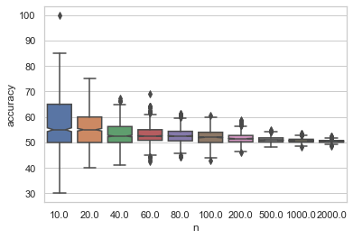
我试图进行一个模拟,其中真正的总体是2类正态分布,两者的平均值为0,标准差为4000。我试图用感知器来确定样本大小与过度拟合程度的关系。然而,感知器总是在6次迭代后收敛,阈值为0,尽管每个类的样本大小为10,但您可以清楚地看到,每个类的阈值不应该是0。为什么阈值总是0?此外,是否有比下面的代码更好地输出阈值的方法?我之所以使用感知器,是因为我想要尽可能简单的分类器--是否有一个更简单、更容易使用的分类器?注意,当以完全相同的方式使用时,Logistic回归似乎有不同于0的阈值。
import numpy as np
mu, sigma = 0, 4000 # mean and standard deviation
pop_size=int(1e4)
p1 = (np.random.normal(mu, sigma, pop_size)) #1 million, pinky
p2 = (np.random.normal(mu, sigma, pop_size))
#take 10 samples of each group and plot on the same plot
def sample_pop(n):
s1 = np.random.choice(p1, size=n, replace=False)
s2 = np.random.choice(p2, size=n, replace=False)
plt.subplot(211)
count, bins, ignored = plt.hist(p1, 50, density=False, color='green', range=[-15000, 15000], histtype='bar', ec='black')
plt.ylabel("n with Rebel Alliance")
ymax=plt.gca().get_ylim()
plt.plot(s1,[ymax]*n,'o',color='green')
plt.subplot(212)
count, bins, ignored = plt.hist(p2, 50, density=False, color = "red", range=[-15000, 15000], histtype='bar', ec='black')
plt.xlabel("Midi Clorian Rate (The Force)")
plt.ylabel("n with Dark Side")
ymax=plt.gca().get_ylim()[1]
plt.plot(s2,[ymax]*n,'x',color='red')
plt.show()
return s1,s2
n=10
s1,s2=sample_pop(n)
from sklearn.linear_model import Perceptron
clf = Perceptron()
s_all=np.hstack((s1,s2)).reshape(-1, 1)
y=np.hstack( ( [0]*len(s1), [1]*len(s2) ) )
clf.fit(s_all, y)
def plot1D(X, y, model,show=True):
# adapted from https://github.com/tirthajyoti/Machine-Learning-with #Python/blob/master/Utilities/ML-Python-utils.py
# Step size of the mesh. Decrease to increase the quality of the VQ.
h = 0.2 # point in the mesh [x_min, m_max]x[y_min, y_max].
# Plot the decision boundary. For that, we will assign a color to each
x_min, x_max = X[:, 0].min() - 1, X[:, 0].max() + 1
y_min, y_max = -.1,.1# X[:, 1].min() - 1, X[:, 1].max() + 1
xx, yy = np.meshgrid(np.arange(x_min, x_max, 0.1),
np.arange(y_min, y_max, 0.1))
# Predictions to obtain the classification results
#Z = model.predict(np.c_[xx.ravel(), yy.ravel()]).reshape(xx.shape)
Z = model.predict(np.arange(x_min, x_max, 0.1).reshape(-1, 1))
dZ=np.diff(Z)
print(Z[np.where(abs(dZ)>0)[0]]) #this is the threshold
# Plotting
if show:
plt.figure(figsize=(6,6))
plt.contourf(xx, yy, np.vstack((Z,Z)), alpha=0.4)
plt.scatter(X[:, 0], np.array( [-.05]*len(X) ), c=y, alpha=0.8, edgecolor="k")
plt.ylim(-.1,0)
plt.gca().get_yaxis().set_ticks([]) #set_visible(False)
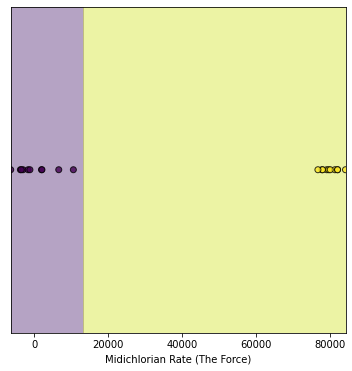
plt.xlabel('Midichlorian Rate (The Force)')
if show:
plt.show()
plot1D(s_all,y,clf)
from sklearn.metrics import accuracy_score
acc=accuracy_score(y, clf.predict(s_all))
acc
clf.n_iter_PS -添加这张图片回答Chris的评论如下:
回答 1
Stack Overflow用户
发布于 2022-07-15 15:38:25
我相信你面临的问题是,由于感知器不可能对两个相同的样本进行正确的分类,无论运行多少次迭代,训练损失都不会改善--模型是随机猜测的。
该模型的默认最小迭代次数为5次,并将继续迭代,直到模型精度改进降到tol阈值以下为止。
在这种情况下,模型在第6次迭代中根本没有改进的可能,因为这是一项不可能的分类任务--所以在第6次迭代之后就结束了。
当模型简化为随机猜测时,我不怀疑您会看到阈值的变化,因为确实没有任何阈值可以可靠地改善分类。
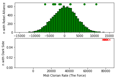
这种行为可以通过将第二个分布移到第一个分布的上界之外、降低tol参数和将max_iter参数增加到更高的数目来证明。
这应该给模型一个战斗的机会。
import numpy as np
import matplotlib.pyplot as plt
mu, sigma = 0, 4000 # mean and standard deviation
pop_size=int(1e4)
p1 = (np.random.normal(mu, sigma, pop_size)) #1 million, pinky
p2 = (np.random.normal(80000, 2000, pop_size))

#take 10 samples of each group and plot on the same plot
def sample_pop(n):
    s1 = np.random.choice(p1, size=n, replace=False)
    s2 = np.random.choice(p2, size=n, replace=False)
    plt.subplot(211)
    count, bins, ignored = plt.hist(p1, 50, density=False, color='green', range=[-15000, 15000], histtype='bar', ec='black')
    plt.ylabel("n with Rebel Alliance")
    ymax=plt.gca().get_ylim()
    plt.plot(s1,[ymax]*n,'o',color='green')
    plt.subplot(212)
    count, bins, ignored = plt.hist(p2, 50, density=False, color = "red", range=[-15000, 15000], histtype='bar', ec='black')
    plt.xlabel("Midi Clorian Rate (The Force)")
    plt.ylabel("n with Dark Side")
    ymax=plt.gca().get_ylim()[1]
    plt.plot(s2,[ymax]*n,'x',color='red')
    plt.show()
    return s1,s2
n=10
s1,s2=sample_pop(n)

from sklearn.linear_model import Perceptron
clf = Perceptron(tol=None, max_iter=20000)
s_all=np.hstack((s1,s2)).reshape(-1, 1)
y=np.hstack( ( [0]*len(s1), [1]*len(s2) ) )
clf.fit(s_all, y)

def plot1D(X, y, model,show=True):

    # adapted from https://github.com/tirthajyoti/Machine-Learning-with #Python/blob/master/Utilities/ML-Python-utils.py

    # Step size of the mesh. Decrease to increase the quality of the VQ.
    h = 0.2    # point in the mesh [x_min, m_max]x[y_min, y_max].

    # Plot the decision boundary. For that, we will assign a color to each
    x_min, x_max = X[:, 0].min() - 1, X[:, 0].max() + 1
    y_min, y_max = -.1,.1# X[:, 1].min() - 1, X[:, 1].max() + 1
    xx, yy = np.meshgrid(np.arange(x_min, x_max, 0.1),
                         np.arange(y_min, y_max, 0.1))
    # Predictions to obtain the classification results
    #Z = model.predict(np.c_[xx.ravel(), yy.ravel()]).reshape(xx.shape)
    Z = model.predict(np.arange(x_min, x_max, 0.1).reshape(-1, 1))
    dZ=np.diff(Z)
    print(Z[np.where(abs(dZ)>0)[0]]) #this is the threshold


    # Plotting
    if show:
        plt.figure(figsize=(6,6))
    plt.contourf(xx, yy, np.vstack((Z,Z)), alpha=0.4)
    plt.scatter(X[:, 0], np.array( [-.05]*len(X) ), c=y, alpha=0.8, edgecolor="k")
    plt.ylim(-.1,0)
    plt.gca().get_yaxis().set_ticks([]) #set_visible(False)
    plt.xlabel('Midichlorian Rate (The Force)')
    if show:
        plt.show()

plot1D(s_all,y,clf)

from sklearn.metrics import accuracy_score
acc=accuracy_score(y, clf.predict(s_all))
acc
clf.n_iter_
https://stackoverflow.com/questions/72993997
复制相似问题
腾讯云开发者

Copyright © 2013 - 2026 Tencent Cloud. All Rights Reserved. 腾讯云 版权所有
深圳市腾讯计算机系统有限公司 ICP备案/许可证号:粤B2-20090059 ![]() 粤公网安备44030502008569号
粤公网安备44030502008569号
腾讯云计算(北京)有限责任公司 京ICP证150476号 | 京ICP备11018762号