雷达系列 | 雷达组网拼图对比教程：PyCWR vs PyCINRAD

用户11172986

发布于 2026-05-07 19:14:13

1210

文章被收录于专栏：气python风雨气python风雨

雷达系列 | 雷达组网拼图对比教程：PyCWR vs PyCINRAD

前言

首先祝大家五一快乐！

3月尾起pycwr突然诈尸更新了许多内容，一看版本更新到1.0.8了，更新了组网插值，风场反演，质量控制之类的功能，没咋细看

打赢复活赛难道是要争夺国内第一雷达库的名头吗

之前很多读者询问过如何绘制雷达组网拼图，也就是radar mosaic

巧妇难为无米之炊，没有多部雷达的数据也谈不上做一期教程

刚好metradar开源的同时给了测试数据，那么我们就开始吧

本教程使用 PyCWR 和 PyCINRAD 两个 Python 库，分别对三个台站的雷达数据进行组网拼图，并对比两者的效果与使用方式。

数据说明

数据源自metradar测试文件

三台站观测时间集中在 2020-06-12 05:39 ~ 05:42 UTC，时间差约 3 分钟，满足组网时间一致性要求。

!pip install pycwr --upgrade --index-url https://pypi.mirrors.ustc.edu.cn/simple/

Successfully installed pycwr-1.0.8

!pip install cinrad --user --upgrade --index-url https://pypi.mirrors.ustc.edu.cn/simple/

Successfully installed cinrad-1.9.3

# 基础库导入
import os
import numpy as np
import xarray as xr
import matplotlib.pyplot as plt
import cartopy.crs as ccrs
import cartopy.feature as cfeature
from glob import glob
# 设置字体（避免中文显示为空白）
plt.rcParams['font.sans-serif'] = ['DejaVu Sans']
plt.rcParams['axes.unicode_minus'] = False

# 数据根目录

BASE_DIR = '/home/mw/project'
RADAR_DIRS = [os.path.join(BASE_DIR, s) for s in ['南京', '泰州', '淮安']]

第一部分：PyCWR 雷达组网

PyCWR 提供了高层封装函数 run_radar_network_3d，可以自动完成：

从每个雷达目录中挑选最接近目标时次的文件
将多部雷达数据插值到统一的经纬度网格
合成 3D 组网反射率体
生成 CR（组合反射率）、VIL（垂直积分液态水含量）、ET（回波顶高）等产品
可选输出为 NetCDF

1.1 运行组网

from pycwr.interp import run_radar_network_3d

# 运行 3D 组网
pycwr_ds = run_radar_network_3d(
    target_time='2020-06-12T05:40:00',      # 目标时次
    radar_dirs=RADAR_DIRS,                   # 每部雷达的目录列表
    lon_min=117.5,                           # 组网区域西边界
    lon_max=121.5,                           # 组网区域东边界
    lat_min=31.0,                            # 组网区域南边界
    lat_max=34.0,                            # 组网区域北边界
    lon_res_deg=0.01,                        # 经向分辨率（约 1km）
    lat_res_deg=0.01,                        # 纬向分辨率（约 1km）
    level_heights=[1000.0, 3000.0, 5000.0],  # 垂直层高度（米）
    field_names=['dBZ'],                     # 组网的场名
    output_products=['CR', 'VIL', 'ET'],     # 附带计算的产品
    composite_method='quality_weighted',     # 合成方法
    max_range_km=460.0,                      # 最大径向距离
    blind_method='hybrid',                   # 盲区处理方法
    parallel=False,                          # 是否并行（首次建议 False）
)

print('Network complete!')
print(pycwr_ds)
print('\nData vars:', list(pycwr_ds.data_vars))
print('Global attrs:', list(pycwr_ds.attrs.keys()))

Network complete!
<xarray.Dataset> Size: 7MB
Dimensions:         (z: 3, lat: 301, lon: 401)
Coordinates:
  * z               (z) float64 24B 1e+03 3e+03 5e+03
  * lat             (lat) float64 2kB 31.0 31.01 31.02 ... 33.98 33.99 34.0
  * lon             (lon) float64 3kB 117.5 117.5 117.5 ... 121.5 121.5 121.5
Data variables:
    dBZ             (z, lat, lon) float64 3MB nan nan nan nan ... nan nan nan
    coverage_count  (z, lat, lon) int16 724kB 0 0 0 0 0 0 0 0 ... 0 0 0 0 0 0 0
    blind_mask      (z, lat, lon) int8 362kB 1 1 1 1 1 1 1 1 ... 1 1 1 1 1 1 1 1
    CR              (lat, lon) float64 966kB 36.85 35.42 34.16 ... 14.9 16.05
    VIL             (lat, lon) float64 966kB 0.2651 0.2333 0.1712 ... nan nan
    ET              (lat, lon) float64 966kB 5e+03 5e+03 5e+03 ... nan nan nan
    ET_TOPPED       (lat, lon) uint8 121kB 1 1 1 1 1 1 1 0 0 ... 0 0 0 0 0 0 0 0
Attributes: (12/32)
    product_type:                    radar_network_3d
    target_time:                     2020-06-12T05:40:00
    radar_count:                     3
    radar_files:                     /home/mw/project/南京/Z_RADR_I_Z9250_20200...
    composite_method:                quality_weighted
    influence_radius_m:              300000.0
    ...                              ...
    output_products:                 ["CR", "VIL", "ET"]
    coverage_policy:                 observable_only
    product_level_heights:           [1000.0, 1500.0, 2000.0, 2500.0, 3000.0,...
    plot_style:                      reference
    plot_canvas_px:                  [920, 790]
    plot_files:                      {}

Data vars: ['dBZ', 'coverage_count', 'blind_mask', 'CR', 'VIL', 'ET', 'ET_TOPPED']
Global attrs: ['product_type', 'target_time', 'radar_count', 'radar_files', 'composite_method', 'influence_radius_m', 'fillvalue', 'projection', 'projection_lon_0', 'projection_lat_0', 'field_range_mode', 'blind_method', 'requested_max_range_km', 'actual_max_range_km_by_field', 'use_qc', 'qc_method', 'qc_clear_air_mode', 'qc_clear_air_max_ref', 'qc_clear_air_max_rhohv', 'qc_clear_air_max_phidp_texture', 'qc_clear_air_max_snr', 'qc_applied_by_radar', 'quality_weight_terms', 'algorithm_references', 'effective_earth_radius', 'network_config_path', 'output_products', 'coverage_policy', 'product_level_heights', 'plot_style', 'plot_canvas_px', 'plot_files']

1.2 查看组网结果

# 查看 CR（组合反射率）
cr_pycwr = pycwr_ds['CR']
print('CR dims:', cr_pycwr.dims)
print('CR valid count:', int((~cr_pycwr.isnull()).sum()), '/', cr_pycwr.size)
print('CR range:', float(cr_pycwr.min().values), '~', float(cr_pycwr.max().values), 'dBZ')

# 查看 VIL 和 ET
if'VIL'in pycwr_ds.data_vars:
    vil = pycwr_ds['VIL']
    print('VIL range:', float(vil.min().values), '~', float(vil.max().values), 'kg/m2')
if'ET'in pycwr_ds.data_vars:
    et = pycwr_ds['ET']
    print('ET range:', float(et.min().values), '~', float(et.max().values), 'km')

CR dims: ('lat', 'lon')
CR valid count: 90352 / 120701
CR range: -10.843102995397057 ~ 68.00083265995372 dBZ
VIL range: 0.00918480371962535 ~ 14.410177000336246 kg/m2
ET range: 1000.1081189278914 ~ 5000.0 km

1.3 PyCWR 组网结果绘图

fig, axes = plt.subplots(1, 2, figsize=(16, 7), subplot_kw={'projection': ccrs.PlateCarree()})

# CR 绘图
ax = axes[0]
cr_pycwr.plot(ax=ax, cmap='jet', vmin=0, vmax=65,
              cbar_kwargs={'label': 'dBZ', 'shrink': 0.8})
ax.set_title('PyCWR Composite Reflectivity (CR)', fontsize=14)
ax.set_xlabel('Longitude')
ax.set_ylabel('Latitude')
ax.add_feature(cfeature.COASTLINE, linewidth=0.5)
ax.add_feature(cfeature.BORDERS, linewidth=0.5)
gl = ax.gridlines(draw_labels=True, linewidth=0.5, color='gray', alpha=0.5, linestyle='--')
gl.top_labels = False
gl.right_labels = False

# VIL 绘图
if'VIL'in pycwr_ds.data_vars:
    ax = axes[1]
    pycwr_ds['VIL'].plot(ax=ax, cmap='YlGnBu', vmin=0, vmax=10,
                         cbar_kwargs={'label': 'kg/m2', 'shrink': 0.8})
    ax.set_title('PyCWR Vertically Integrated Liquid (VIL)', fontsize=14)
    ax.set_xlabel('Longitude')
    ax.set_ylabel('Latitude')
    ax.add_feature(cfeature.COASTLINE, linewidth=0.5)
    ax.add_feature(cfeature.BORDERS, linewidth=0.5)
    gl = ax.gridlines(draw_labels=True, linewidth=0.5, color='gray', alpha=0.5, linestyle='--')
    gl.top_labels = False
    gl.right_labels = False

plt.tight_layout()
plt.show()

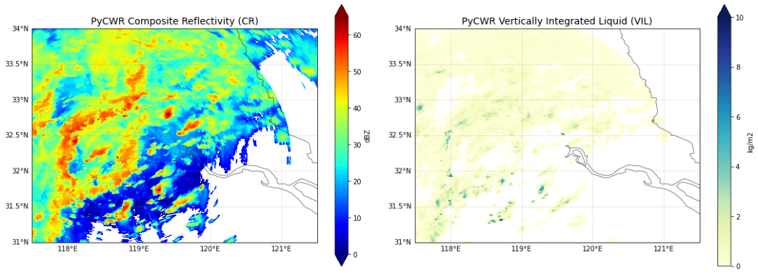
output

第二部分：PyCINRAD 雷达组网

PyCINRAD 提供了 cinrad.calc.GridMapper 类，用于将多部雷达的扫描数据合并到统一的笛卡尔网格上。相比 PyCWR 的自动 3D 组网，PyCINRAD 的组网方式更加底层和灵活，需要用户：

手动读取每部雷达的数据
将极坐标数据转换为笛卡尔坐标（polar_to_xy）
使用 GridMapper 进行网格合并

2.1 读取单站数据并查看信息

import cinrad

station_names = ['Nanjing', 'Taizhou', "Huai'an"]
station_dirs = ['南京', '泰州', '淮安']
radar_data = {}

for station, sdir in zip(station_names, station_dirs):
    f = os.path.join(BASE_DIR, sdir)
    files = [os.path.join(f, x) for x in os.listdir(f) if x.endswith('.bz2')]
    r = cinrad.io.read_auto(files[0])
    radar_data[station] = r
    print(f"{station} ({r.code}): lon={r.stationlon:.3f}, lat={r.stationlat:.3f}, "
          f"scan_time={r.scantime}, ntilts={r.get_nscans()}")

print('\nData read complete!')

Nanjing (Z9250): lon=118.697, lat=32.191, scan_time=2020-06-12 05:42:29+00:00, ntilts=11
Taizhou (Z9523): lon=119.994, lat=32.558, scan_time=2020-06-12 05:40:32+00:00, ntilts=11
Huai'an (Z9517): lon=118.826, lat=33.243, scan_time=2020-06-12 05:39:20+00:00, ntilts=11

Data read complete!

2.2 单仰角（0.5°）基本反射率拼图

# 读取 0.5° 仰角数据并转为笛卡尔坐标
all_br = []
for station in station_names:
    r = radar_data[station]
    br = r.get_data(0, 230, 'REF')           # 0 = 最低仰角，230km 探测距离
    br_xy = cinrad.calc.polar_to_xy(br)      # 极坐标 -> 笛卡尔坐标
    all_br.append(br_xy)
    print(f"{station}: REF shape={br['REF'].shape}, xy grid shape={br_xy['REF'].shape}")

# 使用 GridMapper 拼图
gm_br = cinrad.calc.GridMapper(all_br)
grid_br = gm_br(step=0.01)                   # 0.01° 网格步长

print('\nMosaic complete!')
print(grid_br)
print(f"Valid count: {int((~grid_br['REF'].isnull()).sum())} / {grid_br['REF'].size}")

Nanjing: REF shape=(366, 920), xy grid shape=(1000, 1000)
Taizhou: REF shape=(366, 230), xy grid shape=(1000, 1000)
Huai'an: REF shape=(366, 230), xy grid shape=(1000, 1000)

Mosaic complete!
<xarray.Dataset> Size: 3MB
Dimensions:    (latitude: 521, longitude: 622)
Coordinates:
  * latitude   (latitude) float64 4kB 30.12 30.13 30.14 ... 35.3 35.31 35.32
  * longitude  (longitude) float64 5kB 116.2 116.3 116.3 ... 122.4 122.5 122.5
Data variables:
    REF        (latitude, longitude) float64 3MB nan nan nan nan ... nan nan nan
Attributes:
    elevation:        0
    range:            230
    scan_time:        2020-06-12 05:40:47
    site_code:        RADMAP
    site_name:        RADMAP
    tangential_reso:  nan
    task:             VCP21D
Valid count: 133452 / 324062

/home/mw/.local/lib/python3.9/site-packages/cinrad/calc.py:477: RuntimeWarning: All-NaN axis encountered
  r_data_max = np.nanmax(r_data, axis=0)

2.3 组合反射率（CR）拼图

PyCINRAD 官方计算 CR 的方式是：

rl = list(f.iter_tilt(230, 'REF'))  
cr = cinrad.calc.quick_cr(rl)

然而 cinrad.calc.quick_cr 在 v1.9.3 中存在 bug，下面是根因分析。

Bug 源码

quick_cr 被 @require(["REF"]) 装饰。该装饰器的源码（来自 cinrad/calc.py）如下：

def require(var_names: List[str]) -> Callable:  
    def wrap(func: Callable) -> Callable:  
        @wraps(func)  
        def deco(*args, **kwargs) -> Any:  
            # ... 校验逻辑 ...  
            return func(*args, **kwargs)  

        return wrap    # <-- BUG！应该是 `return deco`  

    return wrap

错误所在：wrap 返回了 wrap（自身）而不是 deco。 后果： 装饰后 quick_cr 实际上是内层的 wrap 函数，而不是 deco。因此当你调用：

cr = cinrad.calc.quick_cr(rl)

quick_cr 执行的是 wrap(rl)，它运行完校验逻辑后 ... 再次返回 wrap（一个函数对象），而不是返回 func(*args, **kwargs)（真正的 CR Dataset）。

正确的装饰器应该怎么写

def require(var_names: List[str]) -> Callable:  
    def wrap(func: Callable) -> Callable:  
        @wraps(func)  
        def deco(*args, **kwargs) -> Any:  
            # ... 校验逻辑 ...  
            return func(*args, **kwargs)  
        return deco    # <-- 正确  
    return wrap

本 notebook 采用的 workaround

由于上游 bug 在 v1.9.3（最新版）中仍然存在，我们绕过损坏的装饰器直接调用核心逻辑。下面的代码单元定义了 quick_cr_fixed，复现了原版 quick_cr 本应使用的内部算法（grid_2d + np.nanmax）。

from xarray import DataArray, Dataset
from cinrad.grid import grid_2d

# 修复版 quick_cr，绕过 cinrad 1.9.3 的装饰器 bug
def quick_cr_fixed(r_list, resolution=(1000, 1000)):
    r_data = []
    r, x, y = grid_2d(
        r_list[0]["REF"].values,
        r_list[0]["longitude"].values,
        r_list[0]["latitude"].values,
        resolution=resolution,
    )
    r_data.append(r)
    for i in r_list[1:]:
        r, x, y = grid_2d(
            i["REF"].values,
            i["longitude"].values,
            i["latitude"].values,
            x_out=x,
            y_out=y,
            resolution=resolution,
        )
        r_data.append(r)
    cr = np.nanmax(r_data, axis=0)
    ret = Dataset({"CR": DataArray(cr, coords=[y, x], dims=["latitude", "longitude"])})
    ret.attrs = i.attrs
    ret.attrs["elevation"] = 0
    return ret

all_cr = []
for station in station_names:
    r = radar_data[station]
    rl = list(r.iter_tilt(230, 'REF'))
    cr = quick_cr_fixed(rl)
    all_cr.append(cr)
    print(f"{station} CR valid pixels: {int((~cr['CR'].isnull()).sum().values)} / {cr['CR'].size}")

# CR 拼图
gm_cr = cinrad.calc.GridMapper(all_cr)
grid_cr = gm_cr(step=0.01)

print('\nCR mosaic complete!')
print(f"Valid count: {int((~grid_cr['CR'].isnull()).sum())} / {grid_cr['CR'].size}")
print(f"Value range: {float(grid_cr['CR'].min().values):.2f} ~ {float(grid_cr['CR'].max().values):.2f} dBZ")

/tmp/ipykernel_268/827592994.py:24: RuntimeWarning: All-NaN axis encountered
  cr = np.nanmax(r_data, axis=0)

Nanjing CR valid pixels: 396782 / 1000000

/tmp/ipykernel_268/827592994.py:24: RuntimeWarning: All-NaN axis encountered
  cr = np.nanmax(r_data, axis=0)

Taizhou CR valid pixels: 460866 / 1000000
Huai'an CR valid pixels: 447054 / 1000000

CR mosaic complete!
Valid count: 145250 / 324062
Value range: 0.10 ~ 70.25 dBZ

/tmp/ipykernel_268/827592994.py:24: RuntimeWarning: All-NaN axis encountered
  cr = np.nanmax(r_data, axis=0)
/home/mw/.local/lib/python3.9/site-packages/cinrad/calc.py:477: RuntimeWarning: All-NaN axis encountered
  r_data_max = np.nanmax(r_data, axis=0)

2.4 PyCINRAD 组网结果绘图

fig, axes = plt.subplots(1, 2, figsize=(16, 7), subplot_kw={'projection': ccrs.PlateCarree()})

# 单仰角拼图
ax = axes[0]
grid_br['REF'].plot(ax=ax, cmap='jet', vmin=0, vmax=65,
                    cbar_kwargs={'label': 'dBZ', 'shrink': 0.8})
ax.set_title('PyCINRAD 0.5 deg Elevation Mosaic', fontsize=14)
ax.set_xlabel('Longitude')
ax.set_ylabel('Latitude')
ax.add_feature(cfeature.COASTLINE, linewidth=0.5)
ax.add_feature(cfeature.BORDERS, linewidth=0.5)
gl = ax.gridlines(draw_labels=True, linewidth=0.5, color='gray', alpha=0.5, linestyle='--')
gl.top_labels = False
gl.right_labels = False

# CR 拼图
ax = axes[1]
grid_cr['CR'].plot(ax=ax, cmap='jet', vmin=0, vmax=65,
                   cbar_kwargs={'label': 'dBZ', 'shrink': 0.8})
ax.set_title('PyCINRAD Composite Reflectivity Mosaic (CR)', fontsize=14)
ax.set_xlabel('Longitude')
ax.set_ylabel('Latitude')
ax.add_feature(cfeature.COASTLINE, linewidth=0.5)
ax.add_feature(cfeature.BORDERS, linewidth=0.5)
gl = ax.gridlines(draw_labels=True, linewidth=0.5, color='gray', alpha=0.5, linestyle='--')
gl.top_labels = False
gl.right_labels = False

plt.tight_layout()
plt.show()

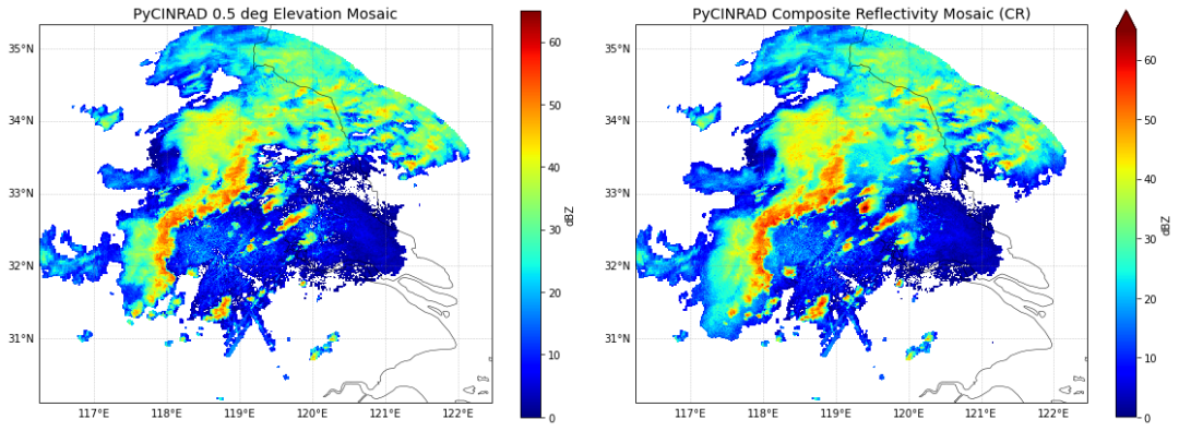
output

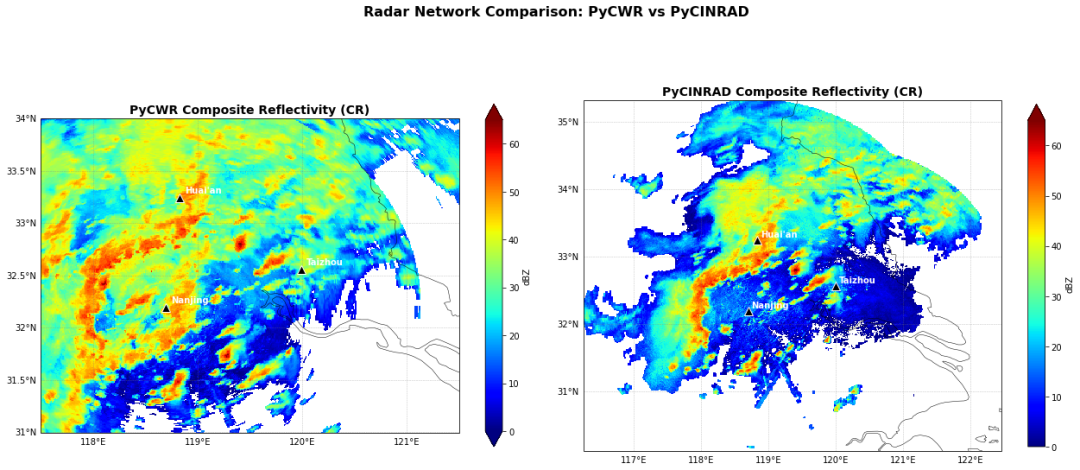
第三部分：效果对比

将 PyCWR 和 PyCINRAD 的 CR 组网结果放在同一张图中进行直观对比。

fig, axes = plt.subplots(1, 2, figsize=(18, 8), subplot_kw={'projection': ccrs.PlateCarree()})

# PyCWR CR
ax = axes[0]
cr_pycwr.plot(ax=ax, cmap='jet', vmin=0, vmax=65,
              cbar_kwargs={'label': 'dBZ', 'shrink': 0.75})
ax.set_title('PyCWR Composite Reflectivity (CR)', fontsize=14, fontweight='bold')
ax.set_xlabel('Longitude')
ax.set_ylabel('Latitude')
ax.add_feature(cfeature.COASTLINE, linewidth=0.5)
ax.add_feature(cfeature.BORDERS, linewidth=0.5)
gl = ax.gridlines(draw_labels=True, linewidth=0.5, color='gray', alpha=0.5, linestyle='--')
gl.top_labels = False
gl.right_labels = False


# PyCINRAD CR
ax = axes[1]
grid_cr['CR'].plot(ax=ax, cmap='jet', vmin=0, vmax=65,
                   cbar_kwargs={'label': 'dBZ', 'shrink': 0.75})
ax.set_title('PyCINRAD Composite Reflectivity (CR)', fontsize=14, fontweight='bold')
ax.set_xlabel('Longitude')
ax.set_ylabel('Latitude')
ax.add_feature(cfeature.COASTLINE, linewidth=0.5)
ax.add_feature(cfeature.BORDERS, linewidth=0.5)
gl = ax.gridlines(draw_labels=True, linewidth=0.5, color='gray', alpha=0.5, linestyle='--')
gl.top_labels = False
gl.right_labels = False

plt.suptitle('Radar Network Comparison: PyCWR vs PyCINRAD', fontsize=16, fontweight='bold', y=1.02)
plt.tight_layout()
plt.show()

output

3.1 统计对比

def stats(da, name):
    vals = da.values.flatten()
    vals = vals[~np.isnan(vals)]
    print(f"{name}:")
    print(f"  Valid pixels: {len(vals)} / {da.size}")
    print(f"  Min: {vals.min():.2f} dBZ")
    print(f"  Max: {vals.max():.2f} dBZ")
    print(f"  Mean: {vals.mean():.2f} dBZ")
    print(f"  Median: {np.median(vals):.2f} dBZ")
    print(f"  Std: {vals.std():.2f} dBZ")
    print()

stats(cr_pycwr, 'PyCWR CR')
stats(grid_cr['CR'], 'PyCINRAD CR')

# 提取重叠区域进行对比
lon_slice = slice(grid_cr.longitude.min().values, grid_cr.longitude.max().values)
lat_slice = slice(grid_cr.latitude.min().values, grid_cr.latitude.max().values)
cr_pycwr_cropped = cr_pycwr.sel(lon=lon_slice, lat=lat_slice)

# 统一坐标名称后插值
cr_pycwr_cropped = cr_pycwr_cropped.rename({'lon': 'longitude', 'lat': 'latitude'})
cr_pycwr_interp = cr_pycwr_cropped.interp(
    longitude=grid_cr.longitude.values,
    latitude=grid_cr.latitude.values,
    method='linear'
)

diff = cr_pycwr_interp - grid_cr['CR']
diff_vals = diff.values.flatten()
diff_vals = diff_vals[~np.isnan(diff_vals)]

print('Overlap difference stats (PyCWR - PyCINRAD):')
print(f"  Valid pixels: {len(diff_vals)}")
print(f"  Mean diff: {diff_vals.mean():.2f} dBZ")
print(f"  Diff std: {diff_vals.std():.2f} dBZ")
print(f"  Max positive diff: {diff_vals.max():.2f} dBZ")
print(f"  Max negative diff: {diff_vals.min():.2f} dBZ")

PyCWR CR:
  Valid pixels: 90352 / 120701
  Min: -10.84 dBZ
  Max: 68.00 dBZ
  Mean: 29.23 dBZ
  Median: 30.85 dBZ
  Std: 12.29 dBZ

PyCINRAD CR:
  Valid pixels: 145250 / 324062
  Min: 0.10 dBZ
  Max: 70.25 dBZ
  Mean: 21.30 dBZ
  Median: 20.53 dBZ
  Std: 13.12 dBZ

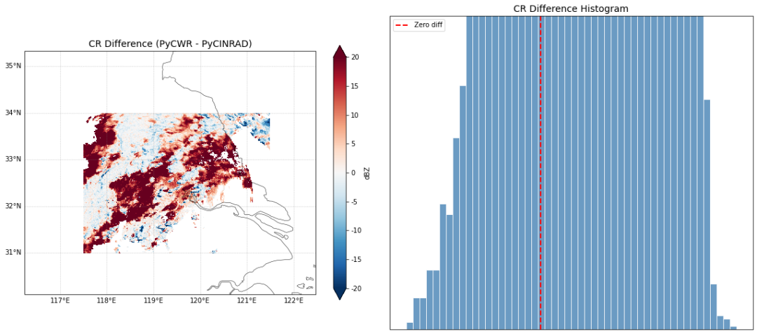
Overlap difference stats (PyCWR - PyCINRAD):
  Valid pixels: 79944
  Mean diff: 8.27 dBZ
  Diff std: 12.58 dBZ
  Max positive diff: 56.21 dBZ
  Max negative diff: -38.59 dBZ

3.2 差异分布图

fig, axes = plt.subplots(1, 2, figsize=(16, 7), subplot_kw={'projection': ccrs.PlateCarree()})

# 差异图
ax = axes[0]
diff.plot(ax=ax, cmap='RdBu_r', vmin=-20, vmax=20,
          cbar_kwargs={'label': 'dBZ', 'shrink': 0.8})
ax.set_title('CR Difference (PyCWR - PyCINRAD)', fontsize=14)
ax.set_xlabel('Longitude')
ax.set_ylabel('Latitude')
ax.add_feature(cfeature.COASTLINE, linewidth=0.5)
ax.add_feature(cfeature.BORDERS, linewidth=0.5)
gl = ax.gridlines(draw_labels=True, linewidth=0.5, color='gray', alpha=0.5, linestyle='--')
gl.top_labels = False
gl.right_labels = False

# 差异直方图
ax = axes[1]
ax.hist(diff_vals, bins=50, color='steelblue', edgecolor='white', alpha=0.8)
ax.axvline(0, color='red', linestyle='--', linewidth=2, label='Zero diff')
ax.set_xlabel('Difference (dBZ)', fontsize=12)
ax.set_ylabel('Count', fontsize=12)
ax.set_title('CR Difference Histogram', fontsize=14)
ax.legend()
ax.grid(True, alpha=0.3)

plt.tight_layout()
plt.show()

output

第四部分：方法对比总结

对比维度	PyCWR	PyCINRAD
使用难度	高封装，一行代码完成组网	低封装，需手动处理每部雷达
3D 组网	原生支持，可生成 3D 反射率体	主要支持 2D 拼图
产品生成	内置 CR、VIL、ET 等产品	quick_cr 等函数当前版本有 bug，需手动实现
自动选时	按 target_time 自动匹配最近文件	需手动指定文件
网格插值	内置 3D 插值到统一经纬度网格	使用 polar_to_xy + GridMapper
质量控制	支持 use_qc=True 自动 QC	需手动处理
输出格式	支持 NetCDF 输出	需手动调用 xarray 输出
灵活性	较低，按固定流程执行	较高，可自定义每一步
性能	支持 parallel=True 并行	单线程，数据量小时足够

差异来源分析

插值算法不同：PyCWR 使用 3D 体积插值，PyCINRAD 使用 2D 平面插值（polar_to_xy 后 GridMapper 合并），导致格点值存在差异。
网格范围不同：PyCWR 的网格由用户指定 (lon_min/max, lat_min/max)，PyCINRAD 的网格由雷达覆盖范围自动确定，两者覆盖区域不完全一致。
CR 计算方式不同：PyCWR 在 3D 体积上取各高度层最大值后投影到地面；PyCINRAD 示例中是在 2D 网格上逐层插值后取最大，插值顺序的差异会导致结果不同。
盲区/范围处理：PyCWR 有 blind_method 和 composite_method 参数控制盲区与合成策略，PyCINRAD 的 GridMapper 使用简单的最近邻/最大值合并。

使用建议

快速业务化组网：推荐 PyCWR，配置简单，产品齐全，适合批量生产。
科研定制分析：推荐 PyCINRAD，每一步可控，便于针对特定算法进行改进和验证。
两个库可以互补使用：用 PyCINRAD 读取和预处理单站数据，用 PyCWR 做高层组网产品生成。

附录：保存结果到 NetCDF

# 保存 PyCWR 结果
pycwr_ds.to_netcdf(os.path.join(BASE_DIR, 'pycwr_network_result.nc'))
print('PyCWR result saved: pycwr_network_result.nc')

# 保存 PyCINRAD CR 结果
grid_cr.to_netcdf(os.path.join(BASE_DIR, 'pycinrad_network_cr.nc'))
print('PyCINRAD CR result saved: pycinrad_network_cr.nc')

# 验证读取
ds_check = xr.open_dataset(os.path.join(BASE_DIR, 'pycinrad_network_cr.nc'))
print('\nVerify PyCINRAD result:')
print(ds_check)

PyCWR result saved: pycwr_network_result.nc
PyCINRAD CR result saved: pycinrad_network_cr.nc

Verify PyCINRAD result:
<xarray.Dataset>
Dimensions:    (latitude: 521, longitude: 622)
Coordinates:
  * latitude   (latitude) float64 30.12 30.13 30.14 30.15 ... 35.3 35.31 35.32
  * longitude  (longitude) float64 116.2 116.3 116.3 116.3 ... 122.4 122.5 122.5
Data variables:
    CR         (latitude, longitude) float64 ...
Attributes:
    elevation:        0
    range:            230
    scan_time:        2020-06-12 05:40:47
    site_code:        RADMAP
    site_name:        RADMAP
    tangential_reso:  nan
    task:             VCP21D

本文参与腾讯云自媒体同步曝光计划，分享自微信公众号。

原始发表：2026-04-30，如有侵权请联系 cloudcommunity@tencent.com 删除

产品