课前准备--Stereo-seq(HD)细胞类型的分布梯度
原创
课前准备--Stereo-seq(HD)细胞类型的分布梯度
原创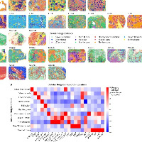
追风少年i
修改于 2026-05-22 10:17:12
修改于 2026-05-22 10:17:12
作者,Evil Genius
今天我们更新思路,针对华大的Stereo-seq。
目前关于华大Stereo-seq的数据分析生态也在慢慢建立,越来越完善,对大家来讲,这是好事。
整体而言,Stereo-seq与HD的分析思路非常接近,都是细胞分割模式 + bin模式。
目前对于空转,高精度和高通量还是有点不可兼得,从大多数的选择来看,选择高精度的多一点。
今天我们更新脚本,以肿瘤细胞为例,实现细胞类型的分布梯度分析。

这个让我想起了,以前做分析的时候,老师要求绘图,我当时真的以为就是绘图,数据准备好了,等老师把数据发过来才发现,是原始数据,什么都没做,要从基础分析开始,背后还需要进行大量的数据分析才能绘图,现在大家都学聪明了,分析之前先开会,沟通思路和现状,完全了解清楚了之后再开始分析。
做这个分析也是一样的,背后需要很多的分析处理。
第一步:选择分析模式,bin还是cellbin?推荐cellbin。
第二步:基础分析,就是基础质控,基因表达太低的细胞是要被去除的。
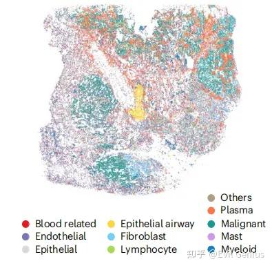
第三步:细胞注释,目前而言,细胞分割模式下无论是Stereo-seq还是HD数据,仍然无法直接用marker注释,还是需要借助单细胞的力量,以匹配的单细胞数据为参考,进行细胞注释,如果看过我之前的文章应该知道分析策略,尤其对于注释不到的细胞,能去除尽量去除。
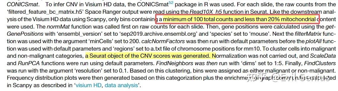
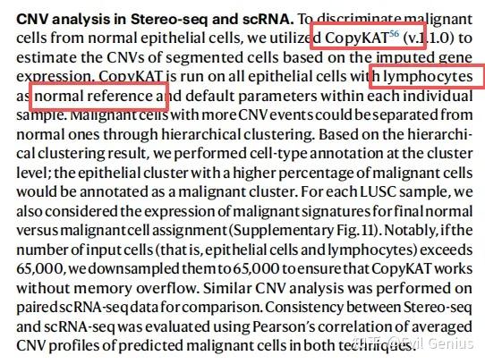
第四步:肿瘤细胞的识别,对于单细胞空间数据而言,肿瘤细胞的识别更多借助的是CNV分析,那么Stereo-seq(HD)在细胞分割模式下可以进行CNV分析么?
有文献作为例证
copycat的代码相对简单,主要分析函数是
copykat.test <- copykat(rawmat=exp.rawdata,
                        id.type="S", # S是symbol的含义
                        ngene.chr=5, # 规定每条染色体中至少5个基因来计算DNA拷贝数(可调整)
                        win.size=25, # 每个片段至少25个基因
                        KS.cut=0.1, # 增加KS.cut会降低敏感度,通常范围在0.05-0.15
                        sam.name="241016",  # 自行命名
                        distance="euclidean",
                        norm.cell.names="",
                        output.seg="FLASE",
                        plot.genes="TRUE",
                        genome="hg20",
                        n.cores=8)
那么在这个基础上,才能做一下个性化的分析,例如我们的细胞类型分布梯度。
第五步:计算梯度(距离需要根据课题设定)
为了定义肿瘤-基质边界,计算每个基质细胞到肿瘤区域内最近恶性细胞的欧氏距离。然后,根据基质细胞与肿瘤的接近程度,以75微米为距离间隔,将其划分为不同的空间层。具体划分如下:位于肿瘤边界0-75微米、75-150微米和150-225微米范围内的基质细胞分别被定义为外层1、外层2和外层3。距离肿瘤边界≥225微米的基质细胞则归为远端基质。
类似地,对于肿瘤区域内的恶性细胞,计算了它们到位于外层1的基质细胞的最近距离,并按照相同的75微米间隔方案划分肿瘤侧的分层。距基质界面0-75微米、75-150微米和150-225微米范围内的细胞分别被归类为内层1、内层2和内层3,而距离≥225微米的细胞则被划入肿瘤核心区域。完成这些分层定义后,即可统计每个分层中髓系细胞的数量。
这个距离分析,我们用代码实现一下,R语言
library(RcppAnnoy)
library(future.apply)
library(Seurat)
library(ggplot2)
library(dplyr)

BuildTree = function(data, n_trees = 50){
  vector_size = ncol(data)
  a_tree <- new(AnnoyEuclidean, vector_size)
  n_samples = nrow(data)
  for (i in 1:n_samples){
    v = as.vector(as.matrix(data[i,]))
    a_tree$addItem(i - 1, v)
  }
  a_tree$build(n_trees)
  return(a_tree)
}

# ========== 2. 获取最近邻函数 ==========
GetNearestNeighbor = function(seurat_obj, n_trees = 50, n_neigh = 10) {
  data = seurat_obj@meta.data[, c("x", "y")]
  a_tree = BuildTree(data = data, n_trees = n_trees)
  neigh_idx = matrix(nrow = nrow(data), ncol = n_neigh)
  neigh_dist = matrix(nrow = nrow(data), ncol = n_neigh)
  res = future_lapply(1:nrow(data), function(x) {
    nei_list = a_tree$getNNsByItemList(x-1, n_neigh, -1, TRUE)
    nei_list$item = nei_list$item + 1
    return(nei_list)
  })
  for (i in 1:nrow(data)) {
    neigh_idx[i, ] <- res[[i]][[1]]
    neigh_dist[i, ] <- res[[i]][[2]]
  }
  return(list(nn.idx = neigh_idx, nn.dists = neigh_dist))
}


seurat_obj_cell@neighbors$Spatial <- GetNearestNeighbor(seurat_obj = seurat_obj_cell, n_neigh = 50)

# 初始定义:D4区域为Tumor core,其余为Stroma(示例)
tumor_domain_cell_idx <- which(seurat_obj_cell@meta.data[, 'domain'] == "D4")
seurat_obj_cell$Tumor_boundary <- "Stroma"
seurat_obj_cell$Tumor_boundary[tumor_domain_cell_idx] <- "Tumor core"

# ========== 从肿瘤核心向外扩张,定义Outer层 ==========
target_cell_idx <- tumor_domain_cell_idx
target_cell_domain <- "Tumor core"
min_neigh <- 10

for (i in 1:3){
  print(paste("Defining Outer", i))
  target_cell_dist <- seurat_obj_cell@neighbors$Spatial$nn.dists[target_cell_idx, ]
  target_cell_neigh <- seurat_obj_cell@neighbors$Spatial$nn.idx[target_cell_idx, ]

  # 找到距离≤150μm且满足条件的Stroma细胞
  target_cell_dist_200 <- sapply(1:nrow(target_cell_neigh), function(x){
    idx <- which(target_cell_dist[x, ] <= 150)
    neigh <- unlist(target_cell_neigh[x, idx])
    neigh_domain <- seurat_obj_cell@meta.data[neigh, "Tumor_boundary"]
    if (length(which(neigh_domain == "Stroma")) > 0 &&
        length(which(neigh_domain == target_cell_domain)) > min_neigh){
      return(neigh[neigh_domain == "Stroma"])
    } else{
      return(NA)
    }
  })

  target_cell_dist_200_neigh <- unique(unlist(target_cell_dist_200))
  target_cell_dist_200_neigh <- target_cell_dist_200_neigh[!is.na(target_cell_dist_200_neigh)]

  seurat_obj_cell$Tumor_boundary[target_cell_dist_200_neigh] <- paste0("Outer ", i)
  target_cell_idx <- target_cell_dist_200_neigh
  target_cell_domain <- paste0("Outer ", i)
}

# ========== 从Outer 1向内扩张,定义Inner层 ==========
o1_domain_cell_idx <- which(seurat_obj_cell@meta.data[, 'Tumor_boundary'] == "Outer 1")
target_cell_idx <- o1_domain_cell_idx
target_cell_domain <- "Outer 1"

for (i in 1:3){
  print(paste("Defining Inner", i))
  target_cell_dist <- seurat_obj_cell@neighbors$Spatial$nn.dists[target_cell_idx, ]
  target_cell_neigh <- seurat_obj_cell@neighbors$Spatial$nn.idx[target_cell_idx, ]

  # 找到距离≤150μm且满足条件的Tumor core细胞
  target_cell_dist_200 <- sapply(1:nrow(target_cell_neigh), function(x){
    idx <- which(target_cell_dist[x, ] <= 150)
    neigh <- unlist(target_cell_neigh[x, idx])
    neigh_domain <- seurat_obj_cell@meta.data[neigh, "Tumor_boundary"]
    if (length(which(neigh_domain == "Tumor core")) > 0 &&
        length(which(neigh_domain == target_cell_domain)) > min_neigh){
      return(neigh[neigh_domain == "Tumor core"])
    } else{
      return(NA)
    }
  })

  target_cell_dist_200_neigh <- unique(unlist(target_cell_dist_200))
  target_cell_dist_200_neigh <- target_cell_dist_200_neigh[!is.na(target_cell_dist_200_neigh)]

  seurat_obj_cell$Tumor_boundary[target_cell_dist_200_neigh] <- paste0("Inner ", i)
  target_cell_idx <- target_cell_dist_200_neigh
  target_cell_domain <- paste0("Inner ", i)
}

# ========== 设置因子水平 ==========
seurat_obj_cell$Tumor_boundary <- factor(seurat_obj_cell$Tumor_boundary,
  levels = c("Tumor core", "Inner 3", "Inner 2", "Inner 1",
             "Outer 1", "Outer 2", "Outer 3", "Stroma"))
拿到注释好的结果,就可以绘制空间分布图了。
color_boundary <- c("#A71B4BFF", "#E96F02FF", "#F9C25CFF", "#FEFDBEFF",
                    "#81DEADFF", "#00A3B6FF", "#584B9F", "#e9e9e9")

# 绘制带图例的PDF
p <- ggplot(data = seurat_obj_cell@meta.data, aes(x = y, y = x, color = Tumor_boundary)) +
  geom_point(size = 0.01) +
  scale_y_reverse() + coord_equal() +
  theme_bw() +
  theme(panel.grid = element_blank(),
        axis.ticks = element_blank(),
        axis.text = element_blank(),
        axis.title = element_blank(),
        panel.border = element_blank(),
        legend.title = element_blank(),
        legend.key.spacing.y = unit(0.8, "lines"),
        legend.spacing.x = unit(1, "lines"),
        legend.text = element_text(size = 20)) +
  guides(color = guide_legend(override.aes = list(size = 7), byrow = TRUE)) +
  scale_color_manual(values = color_boundary)

ggsave(file.path(out_dir, paste0(seurat_obj_cell@project.name, "_tumor_boundary_spatial_colored.pdf")),
       p, width = 12, height = 10)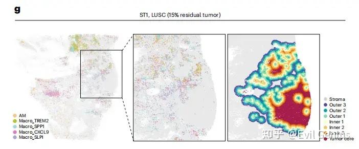
生活很好,有你更好。
原创声明:本文系作者授权腾讯云开发者社区发表,未经许可,不得转载。
如有侵权,请联系 cloudcommunity@tencent.com 删除。
原创声明:本文系作者授权腾讯云开发者社区发表,未经许可,不得转载。
如有侵权,请联系 cloudcommunity@tencent.com 删除。
评论
登录后参与评论
推荐阅读
目录
腾讯云开发者

Copyright © 2013 - 2026 Tencent Cloud. All Rights Reserved. 腾讯云 版权所有
深圳市腾讯计算机系统有限公司 ICP备案/许可证号:粤B2-20090059 ![]() 粤公网安备44030502008569号
粤公网安备44030502008569号
腾讯云计算(北京)有限责任公司 京ICP证150476号 | 京ICP备11018762号