复现升级Cell顶刊：别具风格小提琴图

KS科研分享与服务-TS的美梦

发布于 2026-04-15 18:55:27

粉丝留言，是一篇Cell文章的小提琴图，看起来别具一格，虽然我们没有直接做过这幅图，但是从以往的帖子汲取要点切片，就能够实现这个效果。这里主要四个帖子（复现NC图表：别具一格小提琴图的绘制，复现nature图表：双重组合-渐变背景火山图-效果？无需多言杠杠的！，复现《nature communications》散点小提琴图+蜜蜂图,（群成员专享免费）复现nature图表：ggplot做堆叠小提琴图）。都是基于ggplot2绘图，需要实现小提琴图，添加显著性检验p值，背景渐变颜色等。数据使用的是（https://www.nature.com/articles/s41467-022-32283-3/figures/2）这篇NC文章的数据，原文提供了原始数据。

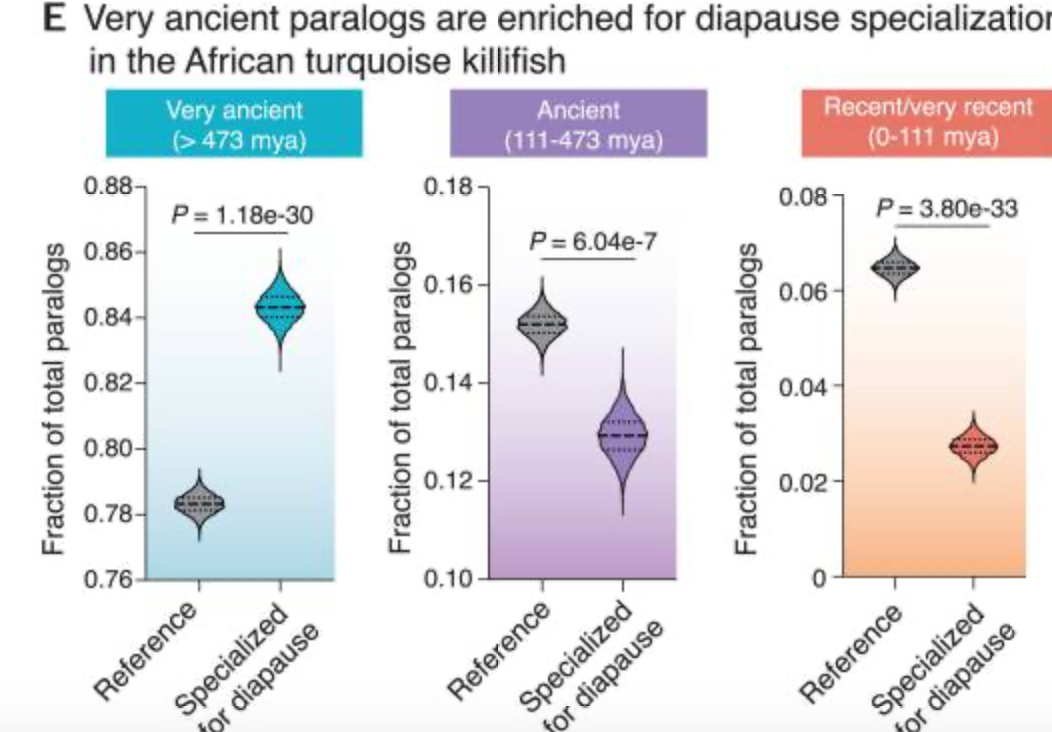
（reference：Singh PP, Reeves GA, Contrepois K, Papsdorf K, Miklas JW, Ellenberger M, Hu CK, Snyder MP, Brunet A. Evolution of diapause in the African turquoise killifish by remodeling the ancient gene regulatory landscape. Cell. 2024 Jun 20;187(13):3338-3356.e30. doi: 10.1016/j.cell.2024.04.048.）

复现效果：

原文提供了数据，下载后处理一下：

setwd("/Users/ks_ts/Documents/公众号文章/复线CELL小提琴图/")
# 安装并加载包
#install.packages("readxl")
library(readxl)
data <- read_excel("./NC_data.xlsx", sheet = 2) #读取第2个sheet的文件
data1 <- data[-1,2:4]
colnames(data1) <- data1[1,]
data1 <- data1[-1,]

#转化为数据框
data1 <- as.data.frame(data1)
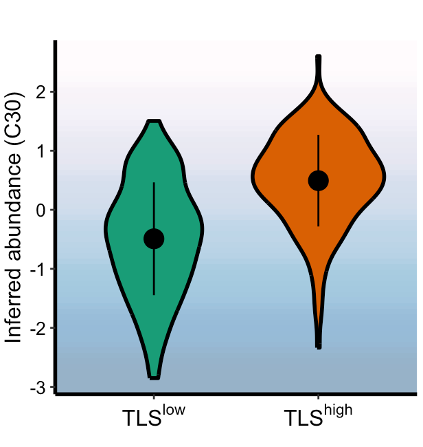
data1$value <- as.numeric(data1$value)

利用之前的代码就可以达到Cell的效果：

library(ggplot2)


rect<- rasterGrob(matrix(alpha(c('#fff7fb','#ece7f2','#d0d1e6','#a6bddb','#74a9cf','#3690c0','#0570b0','#045a8d'),0.5),ncol = 1),
                  width=unit(1,"npc"), height = unit(1,"npc"), interpolate = TRUE) 


ggplot(data1,aes(x=cluster,y=value,fill=cluster))+
  annotation_custom(rect, xmin=-Inf,xmax=Inf,ymin=-Inf,ymax=Inf)+
  geom_violin(width =0.8,color='black',size=1)+#小提请图
  theme_classic() + 
  theme(text = element_text(size=10, colour = "black")) + 
  theme(plot.title = element_text(hjust = 0.5, size = 15),
        axis.text.x = element_text(colour = "black", size = 12),
        axis.text.y = element_text(colour = "black", size = 10),
        axis.title.y = element_text(color = 'black', size = 12),
        axis.line = element_line(size = 1))+ 
  labs(title = "", y = "Inferred abundance (C30)", x=" ") + 
  theme(legend.position="none") +  #不要legend
  stat_summary(fun.data = "mean_sdl",fun.args = list(mult = 1), 
               geom = "pointrange", color = "black", size=1)+#显示中位数和sd，形状为点线形式
  scale_fill_manual(values = c('#1A9E76','#D95F02'))+
  scale_x_discrete(labels=c(expression(TLS^"low"),
                            bquote(TLS^"high"))) #这里说明什么，expression和bquote这两个函数都具有上下标的功能，功能效果一样

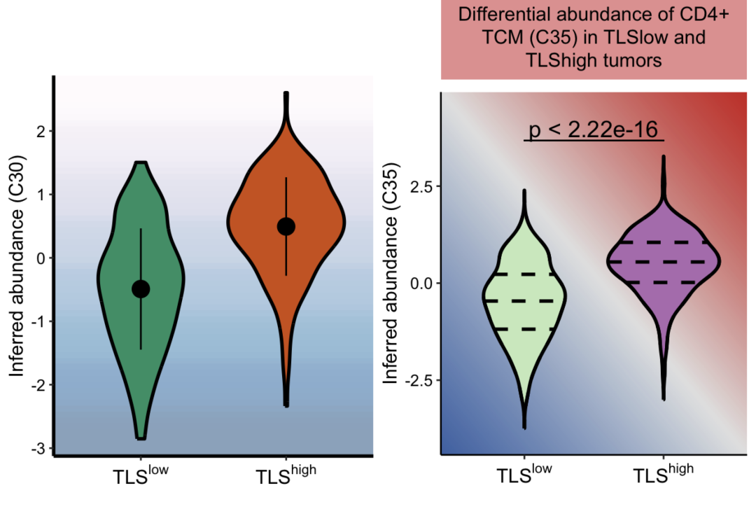
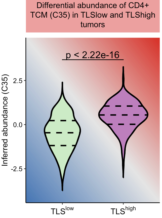
拓展升级一下，两组之间比较，呈现效果趋势无非就是不变化，上升或者下降，所以我们想这个背景的密度梯度可以按照趋势对角线展示：首先设置一个对角线渐变背景颜色函数，可以自定义方向，分辨率，颜色。

set_bgColor <- function(x,
                        res=300,
                        colors=NULL){


  if(is.null(colors)){

    pal <- colorRampPalette(c("#4575b4", "grey90", "#d73027"))
    cols <- pal(256)
  }else{

    pal <- colorRampPalette(colors)
    cols <- pal(256)

  }


  if(x=="increasing"){

    n <- res
    mat <- outer(
      seq(0, 1, length.out = n),
      seq(0, 1, length.out = n),
      function(i, j) ((1 - i) + j) / 2   # 关键改动
    )
  }

  if(x=='decreasing'){

    n <- res  # ‘分辨率’用于生成渐变色背景矩阵，数值越大越
    mat <- outer(
      seq(0, 1, length.out = n),
      seq(0, 1, length.out = n),
      function(i, j) (i + j) / 2)
  }


  # 把矩阵映射到颜色
  mat_scaled <- (mat - min(mat)) / (max(mat) - min(mat))
  img <- matrix(cols[round(mat_scaled * 255) + 1], n, n)


  # 变成 rasterGrob
  g <- rasterGrob(image = img,
                  x = 0.5, 
                  y = 0.5, 
                  width = 1, 
                  height = 1,
                  default.units = "npc",
                  interpolate = TRUE)
  return(g)

}

精细雕琢：

library(ggsignif)
library(ggtext)

#按照升降设置背景
# g <- set_bgColor(x='increasing',
#                  colors = c("white", "grey90", "#d73027"))

g <- set_bgColor(x='increasing')

#添加背景
ggplot(data1,aes(x=cluster,y=value))+
  annotation_custom(
    g,
    xmin = -Inf, xmax = Inf,
    ymin = -Inf, ymax = Inf
  )+
  geom_violin(aes(fill=cluster),
              width =0.8,color='black',size=1,#小提琴图
              trim = F,linetype = "dashed",
              draw_quantiles = c(0.25, 0.5, 0.75))+#展示四分位
  geom_violin(width =0.8,color='black',size=1,fill=NA,trim = F)+
  theme_classic() + 
  theme(text = element_text(size=10, colour = "black"),
        axis.text.x = element_text(colour = "black", size = 12),
        axis.text.y = element_text(colour = "black", size = 10),
        axis.title.y = element_text(color = 'black', size = 12),
        axis.line = element_line(size = 0.5),
        legend.position="none",
        plot.title = element_textbox_simple(
          size = 12,
          padding = margin(5.5, 5.5, 5.5, 5.5),
          margin = margin(0, 0, 15, 0),
          fill = alpha("#d73027",0.5),
          halign =0.5,
        )) + 
  scale_fill_manual(values = c("#CCEBC5",'#BC80BD'))+
  scale_x_discrete(labels=c(expression(TLS^"low"),
                            bquote(TLS^"high")))+
  geom_signif(
    comparisons = list(c("TLS+", "TLS-")),
    test = "t.test",  # 或 "wilcox.test"
    map_signif_level = F,  # TRUE: 显示 *, **, ***; FALSE: 显示 p 值
    textsize = 5,
    tip_length = 0,
    y_position = max(data1$value)+0.8  # 调整显著性标记的高度
  )+
  ylim(-4,4.5)+
  labs(title = "Differential abundance of CD4+ TCM (C35) \n in TLSlow and TLShigh tumors ",
       y = "Inferred abundance (C35)", x=" ")