残差矢量量化(RVQ) : 探索向量优化核心秘密

残差矢量量化(RVQ) : 探索向量优化核心秘密

用户4035096
发布于 2026-07-09 19:07:33
发布于 2026-07-09 19:07:33
残差矢量量化(RVQ) : 探索向量优化核心秘密
残差矢量量化(rvq)是 PostgreSQL 向量索引插件 Vectorchord 提升性能的秘密武器之一. 下面将详细介绍vq, rvq.
以下内容翻译自:
https://drscotthawley.github.io/blog/posts/2023-06-12-RVQ.html
残差矢量量化(RVQ) : 探索“神经音频编解码器”的核心
介绍
“矢量量化”,听起来有点吓人。“残差矢量量化”听起来更吓人,对大多数人来说甚至毫无意义。其实,只要看几张图片,这些概念就很容易理解,甚至连小孩子都能理解——呃……如果小孩子愿意的话。当然,这些算法可以用更复杂的方法实现,我们稍后会稍微介绍一下,但其基础其实非常简单。
残差矢量量化 (RVQ) 是一种数据压缩技术,应用于谷歌SoundStream和 Facebook/Meta AI 的Encodec等先进的神经音频编解码器,而这些编解码器又构成了AudioLM(谷歌)和MusicGen(Facebook)等生成音频模型的支柱。它也被 Lucidrain vector-quantize-pytorch 库应用,由于它速度快且性能好,我们将在最后使用它。
什么是 RVQ?它是如何工作的?
首先,我们应该考虑常规的矢量量化(VQ)。VQ 已经存在了几十年,并且在许多涉及压缩的信号处理领域中都有应用。
注意:每当我说一些同时适用于 VQ 和 RVQ 的内容时,我都会使用缩写“(R)VQ”。
提示:两个类比 1、城市和城镇: RVQ 类似于物流中经常出现的“枢纽辐射”图:以航空旅行为例,主要城市是“枢纽”(芝加哥、洛杉矶、亚特兰大),人们从这些枢纽乘坐小型航班前往较小的城市和城镇。VQ 就像用最近的城镇替换每个地址 —— 这可能会产生大量的向量!RVQ 意味着我们有一个简短的枢纽列表,然后从每个枢纽得到一个较小城市的列表,由此我们可以得到连接较小城市和附近城镇的列表。 2、数字和位数:从某种角度来看,RVQ 类似于我们用位数表示数字的方式。我们不是为从 0 到 9999 的每个整数创建 10,000 个单独的类别,而是使用 4 个“码本”(分别代表千位、百位、十位和个位),每个码本由 0 到 9 这 10 个数字组成。4 * 10 = 40,这比 10,000 少得多!我们甚至可以通过使用更多码本来在小数点右侧包含更小的“残差向量”,从而将实数表示到任意精度。
矢量量化=划分空间
“矢量量化”实际上是将数据点的空间划分成一组离散的区域。换句话说,我们对空间进行了“分区”。
假设我们在空间中有一堆点:
import numpy as np
import matplotlib.pyplot as plt

# make some data
n_points = 25
DATA_MIN, DATA_MAX = -0.5, 0.5 # we'll let these be globals
np.random.seed(9)  # for reproducibility
data = DATA_MIN + (DATA_MAX-DATA_MIN)*np.random.rand(n_points, 2)

# plot it
fig, ax = plt.subplots(figsize=(3,3))
ax.set_xlim(DATA_MIN, DATA_MAX)
ax.set_ylim(DATA_MIN, DATA_MAX)
#ax.set_xticks([])  # hide axis ticks
#ax.set_yticks([])
ax.set_xlabel('x')
ax.set_ylabel('y')
plt.scatter(data[:, 0], data[:, 1], s=16)
plt.show()
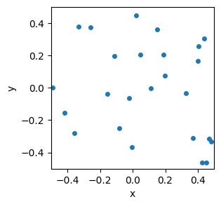
图 1.一组数据点,又称“向量” 。
对于计算机科学家来说,每个点的坐标(x,y)定义了一个“向量”。(对数学家和物理学家来说,“向量”指: 从原点指向每个点,但这种区别对我们来说并不重要。)
澄清 对于神经音频编解码器,向量可以是音频频谱图中的垂直切片(列),即在称为“帧”的短时间间隔内发现的一组频率的振幅列表。然而,更常见的是,向量本身是某些其他音频编码器(例如卷积神经网络)的输出,并且 (R)VQ 是为了进一步压缩这些编码向量,以便执行诸如潜在扩散之类的操作。
现在将空间划分成一堆区域。我们可以采取多种形式来实现这一点。现在,我们先考虑两个例子:
- 我的手绘彩色图和一组平铺的正方形。
- 有一些“更高级”的算法可以以最“拟合”数据的方式划分空间(例如,下文的“k-Means”算法)。
以下abc图式 : 划分或“量化”空间的方法示例,又称“分区方案” 。
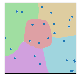
(a)手工
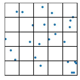
(b)正方形
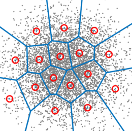
(c)Fancy(图片来源:芬兰阿尔托大学)
图c 为泰森多边形, 参考. 我们稍后可以讨论像图c那样的方案。
- 《PolarDB 开源版 使用PostGIS 以及泰森多边形 解决 "零售、配送、综合体、教培、连锁店等经营"|"通信行业基站建设功率和指向" 的地理最优解问题, 含pgadmin4 容器部署, GIS数据可视化》
- 《重新发现PostgreSQL之美 - 25 最强大脑题目 泰森多边形(空间战略布局问题)》
- 《在PostgreSQL中生成和查看泰森多边形 - Voronoi diagram - 最强大脑题目》
接下来,我可以用squares做更多的代码,所以让我们从那里开始吧。;-)
我稍微形式化一下:我们让变量n_grid控制正方形的数量。因此,对于我们的二维示例,将有n_grid^2方形区域。
通过矢量量化,我们为每个区域赋予一个索引值(例如,对于 5x5 方格,索引值为 0 到 24),然后用该区域的索引替换每个矢量的值。
#| code-fold: true
#| code-summary: "Show the code"
import pandas as pd

def plot_data_grid(data, n_grid=5, hide_tick_labels=True, show_indices=False, show_centroids=False,
                   show_next_level_grid=False):
    "big ol' workhorse plotting routine that we'll progressively make use of as the lesson proceeds"
    fig, ax = plt.subplots(figsize=(3,3))
    h = 1.0 / n_grid
    ax.set_xlim(DATA_MIN, DATA_MAX)
    ax.set_ylim(DATA_MIN, DATA_MAX)

    for i in range(n_grid + 1):
        ax.axhline(DATA_MIN + i*h, color='black')
        ax.axvline(DATA_MIN + i*h, color='black')

    if show_indices:
        index = 0
        for j in range(n_grid):
            for i in range(n_grid):
                x = DATA_MIN + (i + 0.5) / n_grid
                y = DATA_MIN + 1 - (j + 0.5) / n_grid
                ax.text(x, y, str(index), ha='center', va='center',fontsize=14)
                index += 1

    if show_centroids:
        for j in range(n_grid):
            for i in range(n_grid):
                x = DATA_MIN + (i + 0.5)*h
                y = DATA_MIN + (j + 0.5)*h
                ax.plot(x, y, 'ro', markersize=6)

    if hide_tick_labels:
        ax.set_xticks([])
        ax.set_yticks([])

    ax.set_aspect('equal')
    if data is not None:
        plt.scatter(data[:, 0], data[:, 1], s=16)
    plt.show()


n_grid=5
#plot_data_grid(data, n_grid=n_grid)
plot_data_grid(data, n_grid=n_grid, show_indices=True)
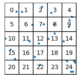
图 3. (0-24整数)每个区域的索引。
对于数据点所代表的每个“向量”,我们不再使用(x,y)坐标对,而是其所在区域的(整数)索引。
笔记 我们已经从每个点需要两个浮点数变成了只需要一个整数值。在二维空间中,由此带来的“节省”或数据压缩量可能并不明显,但请记住:随着我们以后处理大量维度,这种方案将为我们节省大量数据。
如果我们想要与索引对应的坐标,我们将使用每个区域的质心。从这个意义上讲,向量被“量化”,因此它们只能取由区域质心给出的值。在以下示例中,质心显示为红色:
plot_data_grid(data, n_grid=n_grid, show_indices=False,
               show_centroids=True)
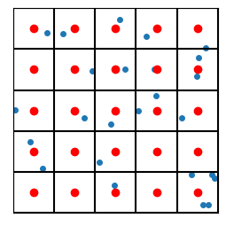
图 4.质心位置
因此,每个蓝点实际上都会被最近的红点替换。从这个意义上讲,我们“量化”了向量(因为我们量化了空间本身)。
术语 质心位置的集合称为“码本”。当我们想要使用(空间中的)实际矢量值时,我们通过查找码本将码本索引转换为(质心)位置。
因此,显示数据点、区域索引和质心的完整(尽管不方便)图片如下所示:
plot_data_grid(data, n_grid=n_grid, show_indices=True, show_centroids=True, hide_tick_labels=False)
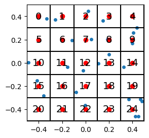
图 5.显示数据点、区域索引和质心位置的详细图表。
对于我们选择的坐标,码本(即索引到质心位置的映射)如下所示:
from IPython.display import display, Markdown

def generate_codebook(n_grid, n_dim=2, debug=False):
    n_gridpoints = n_grid ** n_dim
    if debug: print(f"generate_codebook: n_grid = {n_grid}, n_dim = {n_dim}, n_gridpoints = {n_gridpoints}")
    centroids = np.empty((n_gridpoints, n_dim))
    h = (DATA_MAX - DATA_MIN)/n_grid
    for i in range(n_dim):
        coords = np.linspace(DATA_MIN + h/2, DATA_MAX - h/2, n_grid)
        coords = np.tile(coords, int(n_gridpoints / n_grid ** (i + 1)))
        coords = np.repeat(coords, n_grid ** i)
        centroids[:, i] = coords

    return centroids


codebook = generate_codebook(n_grid)


# print it nicely
cb_str = f"| index      | vector |\n| ----------- | ----------- |"
for i in range(codebook.shape[0]):
    cb_str += f"\n| {i} | ({codebook[i,0]:.1f}, {codebook[i,1]:.1f}) |"
display(Markdown(cb_str))
index | vector |
|---|---|
0 | (-0.4, -0.4) |
1 | (-0.2, -0.4) |
2 | (0.0, -0.4) |
3 | (0.2, -0.4) |
4 | (0.4, -0.4) |
5 | (-0.4, -0.2) |
6 | (-0.2, -0.2) |
7 | (0.0, -0.2) |
8 | (0.2, -0.2) |
9 | (0.4, -0.2) |
10 | (-0.4, 0.0) |
11 | (-0.2, 0.0) |
12 | (0.0, 0.0) |
13 | (0.2, 0.0) |
14 | (0.4, 0.0) |
15 | (-0.4, 0.2) |
16 | (-0.2, 0.2) |
17 | (0.0, 0.2) |
18 | (0.2, 0.2) |
19 | (0.4, 0.2) |
20 | (-0.4, 0.4) |
21 | (-0.2, 0.4) |
22 | (0.0, 0.4) |
23 | (0.2, 0.4) |
24 | (0.4, 0.4) |
重建误差
当我们进行这种量化(即用最近的质心替换向量)时,质心位置与原始数据向量本身相比自然会有些“偏差”。网格越精细,区域越小,误差就越小。对于二维网格在哪里,误差约为h^2, h是网格间距(h = 1/5 = 0.2)。
笔记 请注意,码本中的向量并非“基向量”:我们不会将码本向量进行线性组合,因为那样并非“量化”(并且会将数据点数量与原始数据相同,导致几乎没有压缩)。VQ 通过使用最接近的码本向量来近似数据点,帮助我们解决了数据点数量过多的问题;而 RVQ 中的 R 值则使我们能够在不需要极长码本的情况下,在空间内提供良好的“分辨率”。
让我们检查一下当我们改变网格间距时误差是如何变化的,即当我们改变n_grid时。
def find_closest_centroids(data, codebook):
    distances = np.sum((data[:, np.newaxis] - codebook) ** 2, axis=2)
    closest_centroids = np.argmin(distances, axis=1)
    return closest_centroids # indices not coordinates

def compute_error(data, codebook):
    n_grid = int(np.sqrt(codebook.shape[0]))
    h = 1/n_grid * (DATA_MAX - DATA_MIN)
    quantized_ind = find_closest_centroids(data, codebook)
    quantized_xy = codebook[quantized_ind]
    error = np.sqrt( np.sum( (data - quantized_xy)**2 ) )
    return error

n_points2 = 100
data2 = DATA_MIN + (DATA_MAX - DATA_MIN)*np.random.rand(n_points2, 2)

errors = []
grids = np.array([5,10,25,100,200])
for n_grid2 in grids:
    codebook = generate_codebook(n_grid2)
    error = compute_error(data2, codebook)
    errors.append(error)

fig, ax = plt.subplots(1,2, figsize=(10,4))
ax[0].plot(grids, errors, 'o-')
ax[1].loglog(grids, errors, 'o-')
for i in range(2):
    ax[i].set_ylabel('Error')
    ax[i].set_xlabel('n_grid')
plt.show()
print(f"lowest error (for n_grid={grids[-1]}) = ",errors[-1])
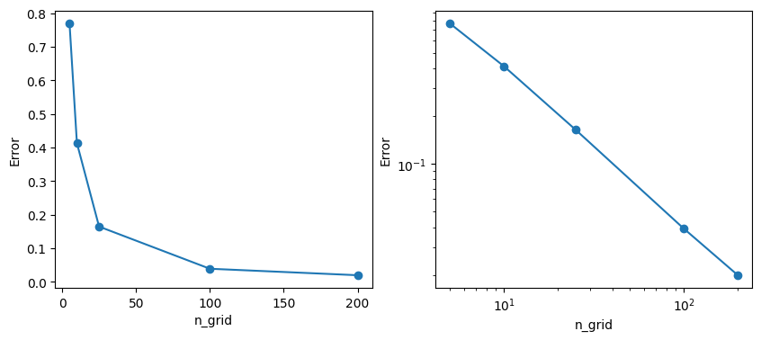
图 6.误差与分辨率的关系图,左轴为线性轴,右轴为对数轴。请注意,计算成本会随着区域数量的增加而变化,即n_grid^2。
lowest error (for n_grid=200) = 0.019903707672610238
所以,使用的“网格线”越多,误差就越小,但代价是什么呢?为了得到 0.02 的误差,我们需要200^2 = 400区域。在高于 2 的维度中,获得更高分辨率/更低误差的“代价”会大幅上升:在D维向量空间中为了将分辨率翻倍,计算成本增加了2^D。(想象D=32、64、128、…)
但我们不需要均匀地覆盖整个空间!这就是残差矢量量化(RVQ)的用武之地。您可以直接跳到RVQ部分。下一部分我们将选一个可选的题外话,学习另一种划分空间的方法,即“k-means”算法。
笔记 另一个关键点:通过替换矢量的所有坐标值(即 浮点数d )为单个整数(网格ID),VQ 实现了数据压缩系数d(浮点数占用的bit数是整数的几倍)。对于大量维度,无论采用何种分区方案,这种压缩都可能非常显著。
k-means 分区方案
关于 k-Means 的讨论实际上对理解 (R)VQ 来说并不重要。完全不是。说实话,完全可以跳过。所以……只有真正好奇才读。否则,直接跳到残差矢量量化部分。
K-Means 算法是另一种划分空间的方法,它取代了静态的正方形,允许我们的区域和质心“跟随数据”动态移动。K-Means 通常用于初始化神经编解码器(例如 SoundStream、Encodec 等)的 RVQ 码本,之后,神经网络的其余训练算法可能会进一步优化码本。
我们将从下面显示的一组数据点开始,这些数据点显示为小黑圈,以及一组用大号彩色圆圈表示的k(“质心”)。(它们现在还不是真正的“质心”,但我们会讲到它)。
# lots of imports to try to get the plotly plots and animations to show!
import plotly.io as pio
pio.renderers.default='notebook'
import plotly.express as px
from plotly.offline import plot, iplot, init_notebook_mode
import plotly.graph_objs as go
init_notebook_mode(connected=True)


ndim = 2  # easier to do in 2d at first
npoints = 100
np.random.seed(1)
datak = DATA_MIN + (DATA_MAX-DATA_MIN)*np.random.rand(npoints, ndim)   # make up some random data points

k = 5        # k-Means parameter: number of clusters

# start with random centroids
centroids = DATA_MIN + 0.2+0.6*(DATA_MAX-DATA_MIN)*np.random.rand(k, ndim) # don't let the starting centroids be on the far edges of the plot
orig_centroids = centroids.copy() # save these for later when we'll make a movie


def plot_kmeans(data, centroids, cluster_memb=None): # we'll leave a way to color the data points
    all_data = np.concatenate((data,centroids))
    is_centroid = np.array( [1 if i >= npoints else 0 for i in range(all_data.shape[0])] , np.newaxis)
    sizes = is_centroid*3 + 1
    cs = cluster_memb if cluster_memb is not None else -1+np.zeros( (data.shape[0],1) ,dtype=int)
    cs = np.append(cs, range(k)) # add the centroids
    plot_data = np.column_stack( (all_data, sizes, cs) )
    columns = ['x','y','sizes','cluster']
    df = pd.DataFrame( plot_data,  columns=columns)
    fig = px.scatter(df, x="x", y="y", color='cluster', size='sizes',  range_color=(-1,k),
            width=420, height=360, color_continuous_scale='Turbo')
    fig.update_layout(margin=dict(l=20, r=20, t=20, b=20),)#template='plotly_dark',)
    return fig

plot_kmeans(datak, centroids)
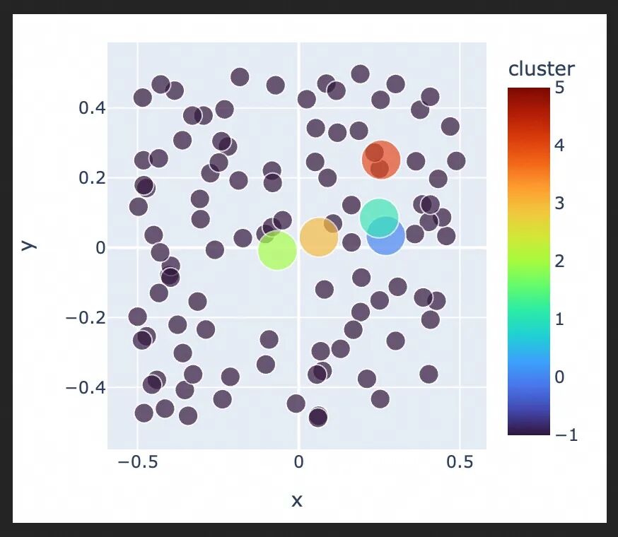
图 7. k-Means 的初始状态,显示没有任何“成员资格”的数据(暗点)和随机质心位置(大彩色点)
这就是我们的起点。接下来,我们要做的是,根据每个点最接近的质心来给它着色。
警告 是的,对于多维空间中的大量点来说,这可能会非常慢。关于如何加速“最近邻”类型的算法,已经有了一套完整的研究体系。在本演示中,我们将尽量简化。接下来,我们将使用的库实际上会进行“近似 K-means”算法来提高速度。
def distance(p1, p2):
    "euclidean distance squared. we don't need the square root b/c we're only interested in ordering by distance"
    return np.sum((p1-p2)**2, axis=1)

def calc_cluster_membership(data, centroids):
    npoints = data.shape[0]
    min_ds = 9999*np.ones(npoints)
    cluster_memb = np.zeros(npoints, dtype=int)-1
    for i, c in enumerate(centroids): # compute distances for all points
        ds = distance(data, c)
        inds = np.argwhere(ds < min_ds)
        if inds.size > 0:
            min_ds[inds] = ds[inds]
            cluster_memb[inds] = i
    assert len(cluster_memb)==npoints # we're not including the centroids themselves here
    return cluster_memb

cluster_memb = calc_cluster_membership(datak, centroids)
plot_kmeans(datak, centroids, cluster_memb=cluster_memb)
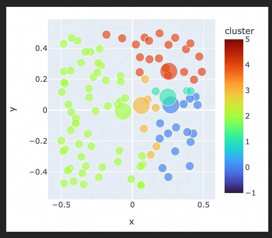
图 8. K-means 聚类的第一步:根据距离质心(大圆点)最近的点,将数据点的“成员”分配到不同的聚类中。请注意,此图中的“质心”还不是真正的质心。我们将在下一步中修复这个问题。
下一步是使用分配给每个质心的点重新计算质心位置。这些质心只是这些点的平均值。
def move_centroids(centroids, data, cluster_memb):
    for ki in range(centroids.shape[0]):
        inds = np.argwhere( cluster_memb == ki)
        if inds.size > 0:
            for dim in range(data.shape[-1]):
                centroids[ki,dim] = np.mean(data[inds,dim], axis=0)
    return centroids

centroids = move_centroids(centroids, datak, cluster_memb)
#print("These centroids should be fairly 'centered' in their respective groups of data.")
plot_kmeans(datak, centroids, cluster_memb=cluster_memb)
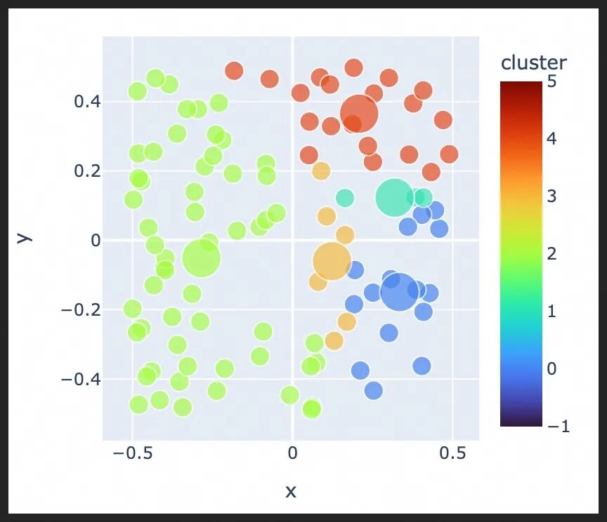
图 9. K-means 算法的下一步:移动质心,使其位于每个聚类的中间
但现在,由于质心移动,一些点的最近邻成员也可能已经改变。因此,我们重新计算这些:
cluster_memb = calc_cluster_membership(datak, centroids)
plot_kmeans(datak, centroids, cluster_memb=cluster_memb)
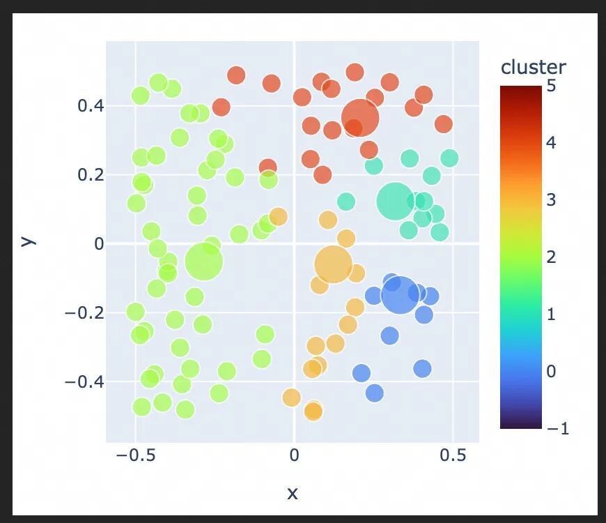
图 10. k-Means 的下一步:根据新的聚类位置重新分配点的聚类成员
… 我们会重复这个过程,直到满足某个停止条件。例如,我们可以设置一个最大迭代次数(vectorchord索引build过程中也有一个参数可设置轮次),或者当质心停止移动,或者聚类成员停止变化时停止,等等。在本演示中,我们将只使用最大迭代次数。
因此,整个过程的电影看起来可能是这样的:
centroids = orig_centroids.copy() # start over
cluster_memb = -1+np.zeros( (datak.shape[0],1) ,dtype=int)
maxiter = 10
plot_kmeans(datak, centroids, cluster_memb=cluster_memb)
ts = np.arange(2*maxiter,dtype=int)

columns = ['t','x','y','sizes','cluster','point_number']
total_points = npoints + k  # points + clusters
movie_data = np.zeros( (len(ts)*total_points, len(columns)) )  # giant data array for all data points at all times
movie_data[:,0] = np.repeat(ts, total_points)          # t

xs = np.concatenate( ( datak[:,0], centroids[:,0] ) ) # initial xs
ys = np.concatenate( ( datak[:,1], centroids[:,1] ) ) # initial ys
movie_data[:,1] = np.tile(xs, len(ts))
movie_data[:,2] = np.tile(ys, len(ts))

sizes = np.ones(total_points,dtype=int)
sizes[-k:] = 3
movie_data[:,3] = np.tile(sizes, len(ts)) # sizes is repeated for all times

cs = -2 + np.ones(total_points,dtype=int)
cs[-k:] = np.arange(k, dtype=int)
movie_data[:,4] = np.tile(cs, len(ts))

movie_data[:,5] = np.tile(np.arange(total_points), len(ts))  # point_number is repeated for all time

for t in ts:
    if t==0:
        continue# leave initial data as step 0
    elif t % 2 == 1:
        cluster_memb = calc_cluster_membership(datak, centroids)
    else:
        centroids = move_centroids(centroids, datak, cluster_memb)

    start, end = t*total_points, (t+1)*total_points
    movie_data[start:end, 1] = np.concatenate( (datak[:,0], centroids[:,0]) )    # xs
    movie_data[start:end, 2] = np.concatenate( (datak[:,1], centroids[:,1]) )    # ys
    movie_data[start:end, 4] = np.concatenate( (cluster_memb, np.arange(k, dtype=int)) )  # cluster membership


df = pd.DataFrame(movie_data, columns=columns)
#df['cluster'] = df['cluster'].astype(int).astype(str) # use discrete colormap
#display(df)


fig = px.scatter(df, x="x", y="y", animation_frame="t", animation_group="point_number",
           color="cluster", hover_name="cluster", hover_data=['point_number'],
           size='sizes', width=420, height=460, range_color=(-1,k), color_continuous_scale='Turbo'
           )
fig.update_layout( margin=dict(l=20, r=20, t=30, b=10),)# template='plotly_dark',)
fig.layout.updatemenus[0].buttons[0].args[1]["transition"]["duration"] = 0 # don't interpolate frames
display(fig)
#print( "Caption: In this movie, each step will either be the 'membership' step or \nthe 'centroid moving' step.")
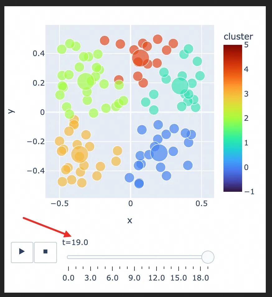
图 11. (交互式)在以上pic中,每个时间步骤要么是根据当前质心计算“集群成员”的步骤,要么是“质心移动”的步骤。
对于那些感兴趣的人,我会在下面放上一个有效的 k-Means 算法的代码——它很短!
def kmeans(data, k=5, n_iter=8):
    n_dim, data_min, data_max = data.shape[-1], np.min(data), np.max(data)
    centroids = data_min + 0.2+0.6*(data_max-data_min)*np.random.rand(k, n_dim) # random init
    for it in range(n_iter):
        cluster_memb = calc_cluster_membership(data, centroids)
        centroids = move_centroids(centroids, data, cluster_memb)

    return centroids, cluster_memb
由于 k-Means 是一种“最近邻”算法,因此它的最终结果是根据“Vornonoi 图”分组的一组向量,如本文开头所示,为了便于说明,我们将再次展示该图:
图 12.通过 k-Means 算法实现的空间划分。( 图片来源:芬兰阿尔托大学 )
残差矢量量化(RVQ)
顺便说一句,RVQ 已经存在很长一段时间了。
基本思想:“码本中的码本”
RVQ 的诀窍在于,它不是使用单个高分辨率码本,而是“码本套着码本”,或者,如果你愿意,也可以称之为“码本堆叠”。假设我们想将初始 5x5 网格的分辨率提高五倍。我们不使用 25x25 网格(这将导致计算成本是原始网格的 25 倍),而是在向量量化的区域“内部”放置一个小的 5x5 网格,结果会怎样?
例如,在“中间”区域(区域 12),我们可以做……
from matplotlib import collections  as mc


def get_region_membership(data:np.array, h=0.2, codebook=None):
    "Tells which region each point is in. TBD: this is slow but it works! ;-) "
    memb = np.zeros(data.shape[0], dtype=np.int32)
    if codebook is None:  # just assume basic squares
        for di, p in enumerate(data):
            i = (p[0]-DATA_MIN) // h
            j = (p[1]-DATA_MIN) // h
            ind = i + j*n_grid
            memb[di] = ind
    else:
        memb = calc_cluster_membership(data, codebook)
    return memb


def plot_data_grid_with_resids(data, n_grid=5, hide_tick_labels=True, show_indices=False, show_centroids=False,
                   show_next_level_grid=False, show_resids=True, codebook=None, show_grid=True):
    "big ol' workhorse plotting routine that we'll progressively make use of as the lesson proceeds"
    fig, ax = plt.subplots(figsize=(3,3))
    h = 1.0 / n_grid
    ax.set_xlim(DATA_MIN, DATA_MAX)
    ax.set_ylim(DATA_MIN, DATA_MAX)

    if show_grid:
        for i in range(n_grid + 1):
            ax.axhline(DATA_MIN + i*h, color='black')
            ax.axvline(DATA_MIN + i*h, color='black')

    if show_next_level_grid: # draws lines in the middle
        x_start = 2*h
        y_start = -h/2
        for i in range(n_grid): # horizontal lines
            y = y_start + i*h/n_grid
            ax.axhline(y, xmin=x_start, xmax=x_start+h, color='black')
        y_start, x_start = x_start, y_start
        for j in range(n_grid): # horizontal lines
            x = x_start + j*h/n_grid
            ax.axvline(x, ymin=y_start, ymax=y_start+h, color='black')

    if show_indices:
        index = 0
        for j in range(n_grid):
            for i in range(n_grid):
                x = DATA_MIN + (i + 0.5) / n_grid
                y = DATA_MIN + 1 - (j + 0.5) / n_grid
                ax.text(x, y, str(index), ha='center', va='center',fontsize=14)
                index += 1

    if show_centroids:
        for j in range(n_grid):
            for i in range(n_grid):
                x = DATA_MIN + (i + 0.5)*h
                y = DATA_MIN + (j + 0.5)*h
                ax.plot(x, y, 'ro', markersize=6)

    if show_resids and codebook is not None:
        memb = get_region_membership(data, codebook=codebook)
        resids = data*0
        lines = []
        for i, p in enumerate(data):
            #resids[i] = p - codebook[memb[i]] # don't actually need to compute resids for this
            lines.append([p, codebook[memb[i]] ] )
        lc = mc.LineCollection(lines, colors=(1,0,1,1), linewidths=2)
        ax.add_collection(lc)

    if hide_tick_labels:
        ax.set_xticks([])
        ax.set_yticks([])

    ax.set_aspect('equal')
    if data is not None:
        plt.scatter(data[:, 0], data[:, 1], s=16)
    plt.show()


n_grid=5
codebook = generate_codebook(n_grid)
plot_data_grid_with_resids(data, n_grid=n_grid, show_next_level_grid=True, show_centroids=True,
                           hide_tick_labels=False, codebook=codebook, show_resids=False)
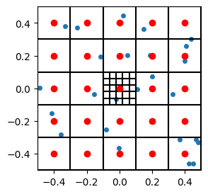
图 13. “码本中的码本”图示,其中较小的 5x5 码本将相对于中间区域的码本。
中间“主”方块中的蓝点与其对应的红色质心之间的差异将成为“残差”。我们也将在“小”5x5网格内对其进行量化。这将作为原始码本“之后”使用的码本。我们将获得与 25x25 网格相同的分辨率,只是计算成本将改为 2*(5*5)=50,而不是 25*25=625!因此,我们的成本将比全网格方法小 12.5 倍。
有趣的是,如果我们只考虑残差,即主质心和所讨论向量之间的差异,那么我们可以对空间中的所有点使用相同的“下一级”码本!在下图中,我们将残差显示为从每个点延伸到其对应的最近质心的紫色线段:
plot_data_grid_with_resids(data, n_grid=n_grid, show_next_level_grid=True, show_centroids=True,
                           hide_tick_labels=True, codebook=codebook, show_resids=True)
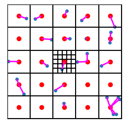
图 14。重新定义的图示,显示为连接向量(蓝点)及其最近的质心(红点)的紫色线段。
此外,因为我们巧妙地将数据设置为以原点为中心(0,0),我们可以将原始数据点视为相对于整个域的“质心”即原点的“残差”!
plot_data_grid_with_resids(data, n_grid=n_grid, show_next_level_grid=False, show_centroids=False,
                           hide_tick_labels=False, codebook=np.zeros((data.shape[0],2)), show_resids=True, show_grid=False)
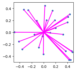
图 15.对于“0 级”码本,我们如何将数据点本身视为相对于原点的残差
同样,由于我们巧妙地选择了坐标,对于下一级量化,我们可以将下一级的码本取为上一级码本除以n_grid!情况并非总是如此;我只是觉得自己很聪明,也很懒。
量化器算法
到目前为止,我们默认隐藏了代码。但为了真正理解 RVQ 方法,我将展示代码。
让我们编写一个通用的、多“层”嵌套码本的量化器。它将获取我们的数据点并返回各层码本的索引。
将遵循 Google 2021 年论文“SoundStream:端到端神经音频编解码器”第 4 页中的“算法 1”:
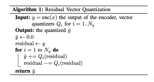
图 16.SoundStream 的 RVQ 算法
但我喜欢我的写作方式:
def quantizer(data, codebooks, n_grid=5):
    "this will spit out indices for residuals in a series of 'nested' codebooks"
    resids = data
    indices = []
    for cb in codebooks:
        indices_l = get_region_membership(resids, codebook=cb)
        resids = resids - cb[indices_l]
        indices.append(indices_l)
    return np.array(indices)

# Make the nested codebooks
n_codebooks = 3
codebook = generate_codebook(n_grid)
codebooks = [codebook/n_grid**level for level in range(n_codebooks)]

indices = quantizer(data, codebooks)   # call the quantizer
display(indices)
array([[10,  2,  5,  7,  5, 20,  4, 13, 19, 17, 16, 14, 24,  4, 22, 23,
         4, 21, 19, 11, 13, 12,  4, 18,  4],
       [10, 17,  3,  5, 17,  9,  3, 22,  7, 13, 14,  5,  3, 24, 18,  6,
        24,  6, 17,  8, 10,  1, 21, 12,  3],
       [11,  6, 12,  7, 15, 20, 23,  7, 17, 13,  8, 18,  2,  7, 15, 11,
        16, 20, 23, 13, 11, 24, 18, 10, 20]])
让我们尝试使用每一级码本重建原始数据来测试一下。下图中,原始数据为蓝色,其他颜色表示使用递增数量的码本进行量化的结果:
K = n_codebooks
fig, ax_all = plt.subplots(nrows=1, ncols=K, figsize=(10+(K-3),3))
recon = data*0
for axi in range(K):
    ax = ax_all[axi]
    ax.scatter(data[:, 0], data[:, 1], s=16)
    recon += codebooks[axi][indices[axi]]
    ax.scatter(recon[:, 0], recon[:, 1], s=16, color='orange')
    ax.set_xticks([])
    ax.set_yticks([])
    hpos = 1/K*0.85 + 1/K*0.81*axi if K==4 else .25 + .27*axi
    fig.text(hpos, .05, f"{axi+1} codebook{'s' if axi>0 else ''}", ha='center')

    error = ((recon - data)**2).mean()
    fig.text(hpos, .0001, f"Error = {error:.2e}", ha='center')

plt.show()
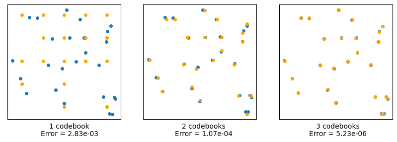
图 17.使用多级RVQ 码本(橙色点)重建数据(蓝色点)
我们发现,使用的码本层数越多,我们就能越准确地逼近原始数据。最右边的图像的有效分辨率为5^3=125小方块,在二维中而是只使用5*5*2=75,这并不是一个巨大的节省,但让我们看看这对于更高维度来说有多重要。
设维度为d,并且K是码本的数量(“与 k-means中的 k 无关”)。我们将用大量数据填充一个 d 维超立方体,并使用 RVQ 将其细分为嵌套的小超立方体组,并计算误差 —— 以及与使用常规 VQ 而不是 RVQ 相比的计算成本“节省”。
笔记 使用均匀的正方形/(
d维)超立方体区域是一个非常愚蠢的想法。因为区域的数量会像n_grid^d,实际上可能比我们拥有的数据向量数量要大得多!我们将在下面尝试一种更复杂的分区方案。
#### label: fig-rvq-recon-highdim2
#### fig-cap: "Error for high-dimensional datasets using various levels of RVQ. 'cost savings factor' refers to the ratio of using regular VQ (at uniform resolution) vs RVQ"

d_choices = [2, 3, 4, 6]  # we can't go much higher with 5x5 uniform grids!
K_choices = [1,2,3,4]     # variable numbers of codebooks

npoints_hd = 1000  # points in high-dim spaces

print("Here we show the error for high-dimensional datasets using various levels of RVQ.")
print("'cost savings factor' refers to the ratio of using regular VQ (at uniform resolution)\nvs RVQ.")

for d in d_choices:
    print(f"\nd = {d}:")
    np.random.seed(1)
    data_hd = DATA_MIN + (DATA_MAX-DATA_MIN)*np.random.rand(npoints_hd, d)
    codebook0 = generate_codebook(n_grid, n_dim=d)
    codebooks = [codebook0/n_grid**level for level in range(max(K_choices))] # lets get this over with rather than in the loop
    for K in K_choices:
        indices = quantizer(data_hd, codebooks)
        recon = data_hd*0
        for lil_k in range(K):   # reconstruct using all codebooks
            recon += codebooks[lil_k][indices[lil_k]]
        error = ((recon - data_hd)**2).mean()
        grid_0_points = n_grid**(d)
        rvq_points = grid_0_points*K
        uni_res = grid_0_points**K # comparable uniform resolution
        savings = uni_res/rvq_points
        print(f"  K = {K}, error = {error:.2e}, cost savings factor = {savings:.1f}")
        pass
Here we show the error for high-dimensional datasets using various levels of RVQ.
'cost savings factor' refers to the ratio of using regular VQ (at uniform resolution)
vs RVQ.

d = 2:
  K = 1, error = 3.41e-03, cost savings factor = 1.0
  K = 2, error = 1.29e-04, cost savings factor = 12.5
  K = 3, error = 5.26e-06, cost savings factor = 208.3
  K = 4, error = 2.16e-07, cost savings factor = 3906.2

d = 3:
  K = 1, error = 3.37e-03, cost savings factor = 1.0
  K = 2, error = 1.29e-04, cost savings factor = 62.5
  K = 3, error = 5.31e-06, cost savings factor = 5208.3
  K = 4, error = 2.18e-07, cost savings factor = 488281.2

d = 4:
  K = 1, error = 3.36e-03, cost savings factor = 1.0
  K = 2, error = 1.32e-04, cost savings factor = 312.5
  K = 3, error = 5.34e-06, cost savings factor = 130208.3
  K = 4, error = 2.16e-07, cost savings factor = 61035156.2

d = 6:
  K = 1, error = 3.37e-03, cost savings factor = 1.0
  K = 2, error = 1.33e-04, cost savings factor = 7812.5
  K = 3, error = 5.35e-06, cost savings factor = 81380208.3
  K = 4, error = 2.16e-07, cost savings factor = 953674316406.2
然而,这些“成本节省因素”是人为设定的,因为我们仍然使用正方形/(d维)超立方体来划分区域,我们不需要那样塑造它们,也不需要那么多。(R)VQ 的优点在于,你可以指定所需的质心数量 —— 也就是你想要的码本有多“长” —— 即使维度数量激增,你也可以将其保持在一个可控的范围内。
因此,为了处理更高的维度,我们需要停止使用均匀的正方形,这样我们就可以得到一个小于几千个质心的码本“长度”(而不是刚才的数十万个,例如 5^8 = 390625)。为了获取跟随数据的非均匀区域,我们将使用上面描述的 k-Means 方法。
让我们看看重建误差在高维度中的表现。
误差分析:指数收敛
我们可以尝试给定数量的(最初)随机质心,并尝试通过 k-Means 将它们与数据匹配。
笔记 RVQ 计算中不同层级的残差可能具有不同的数据分布。这意味着,我们不再像以前那样“共享(缩放的)码本”,而是需要在每个“层级”重新计算一个新的码本。否则,RVQ 不会带来任何优势(相信我,我试过了)。
在下面的计算中,我们将改变维数、码本的长度和码本的数量,看看这些如何影响重建误差。
但是,不要使用我们的代码,而是使用 lucidrains 提供的精彩存储库:lucidrains/vector-quantize-pytorch
以下错误值集合是一堆数字,您可能不感兴趣。您可以随意滚动过去,直接查看(部分)数字的图形表示。
import torch
from vector_quantize_pytorch import ResidualVQ
from functools import partial

def make_pretty(d,styler):
    styler.set_caption(f"d = {d}:")
    styler.format(lambda e: f'{10**e:0.1e}')   # undo the log op
    styler.background_gradient(axis=None, vmin=-12, vmax=1, cmap="plasma")
    return styler

def show_colored_data(results_d, d, cb_lengths, K_choices):
    "displays a dataframe table but colors the background according to log10 of the numbers"
    rdf = pd.DataFrame(np.log10(results_d.numpy()),
                       columns=[f'K = {k}'for k in K_choices],
                       index=[f'cb_len = {c}'for c in cb_lengths])
    ourfunc = partial(make_pretty,d)
    display(rdf.style.pipe(ourfunc))
    return

n_dim = 256  # number of dimensions
cb_len = 256 # codebook length
K = 4        # number of codebooks
npoints_hd = 4096  # number of data points in high-dim space

d_choices = [2, 3, 6, 8, 16, 32, 64, 128, 256, 512]  # dimensions to try
cb_lengths = [25, 64, 256, 1024, 2048]                 # codebook lengths
K_choices = [1,2,3,4,6,8,10]#,16]                           # variable numbers of codebooks

results = torch.empty( ( len(d_choices), len(cb_lengths), len(K_choices) )).cpu()
for q1, n_dim in enumerate(d_choices):
    #print(f"\nd={n_dim:4}:       {' '.join([f'      K={i}' for i in K_choices])}")
    for q2, cb_len in enumerate(cb_lengths):
        #print(f"   cb_len={cb_len:4}: ",end="")
        for q3, K in enumerate(K_choices):

            residual_vq = ResidualVQ(
                dim = n_dim,
                codebook_size = cb_len,
                num_quantizers = K,
                kmeans_init = True,   # set to True
                kmeans_iters = 10     # number of kmeans iterations to calculate the centroids for the codebook on init
            )
            torch.manual_seed(0)
            x = torch.randn(1, npoints_hd, n_dim)
            quantized, indices, commit_loss = residual_vq(x)
            error = ((quantized - x)**2).mean()
            #print(f"  {error:.1e} ", end="")
            results[q1,q2,q3] = error
        #print()
    show_colored_data(results[q1], n_dim, cb_lengths, K_choices)
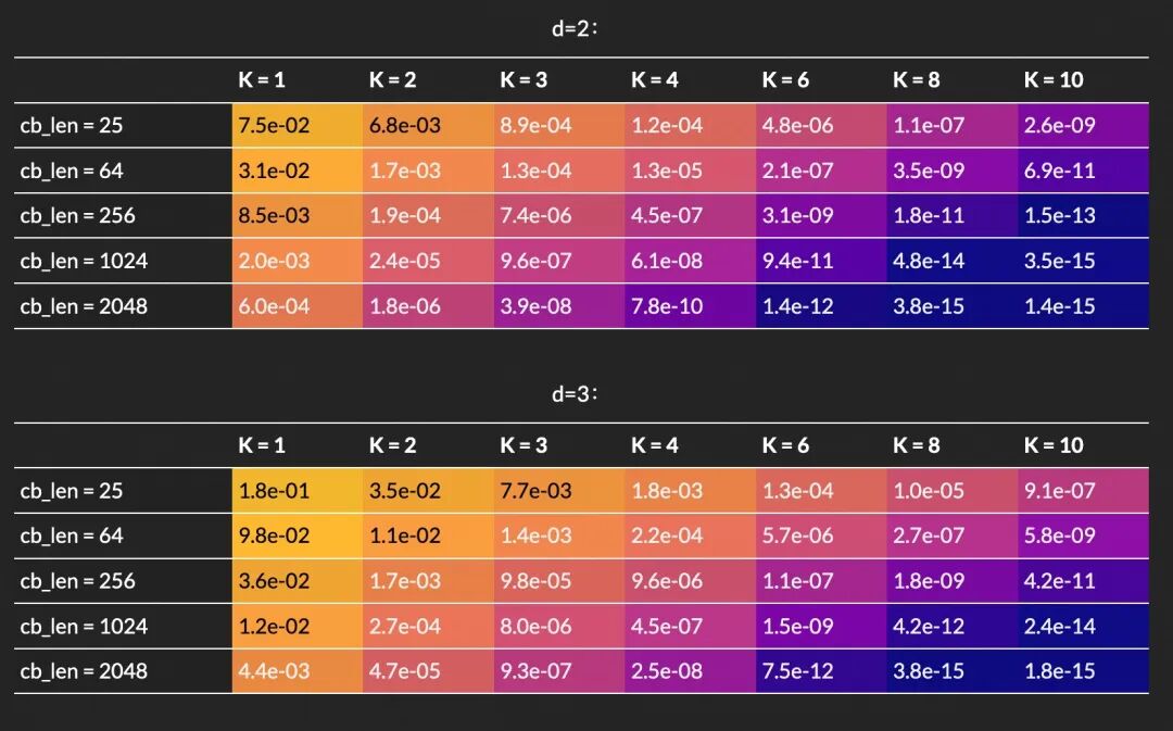
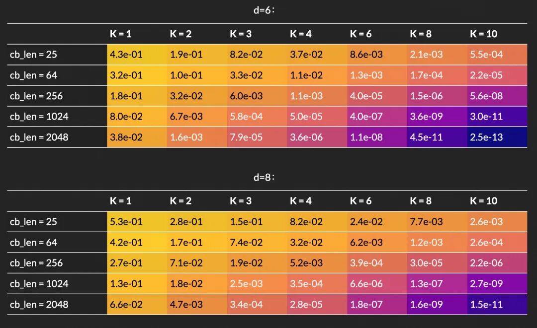
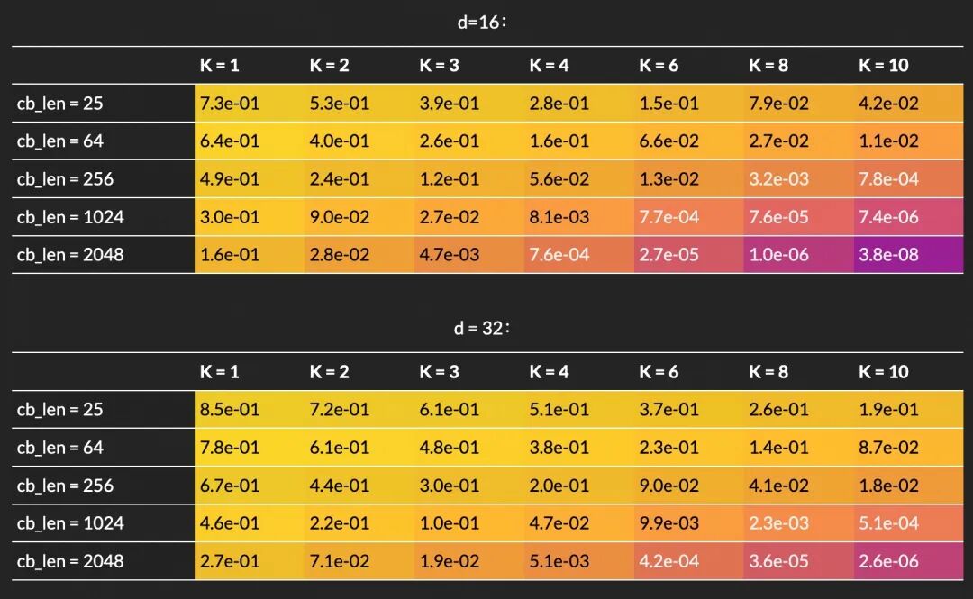
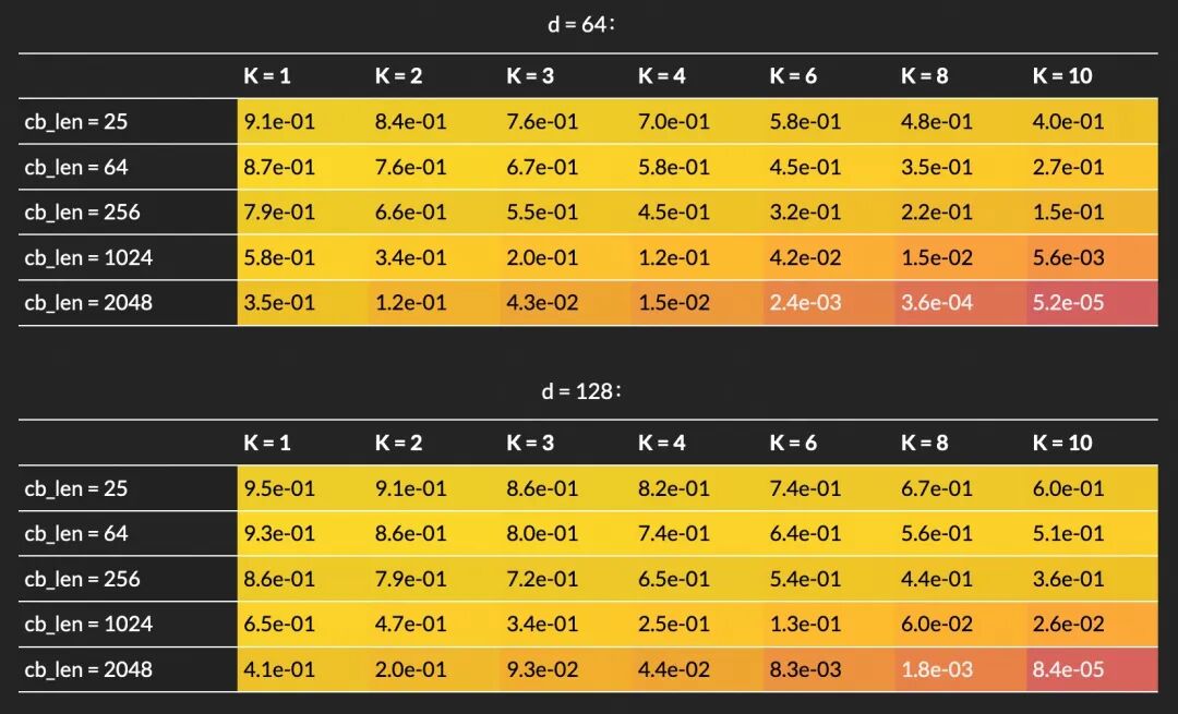
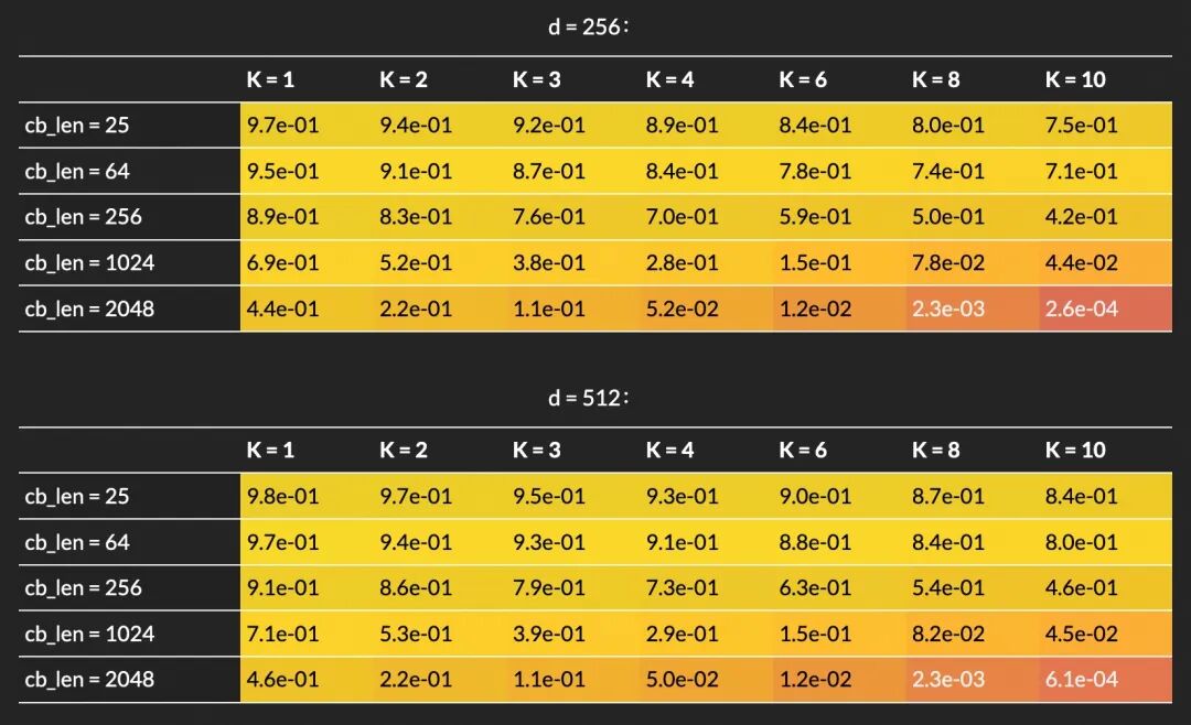
澄清:
K=1的 RVQ 与常规 VQ 相同。
import numpy as np
import plotly.graph_objects as go
import plotly.io as pio
pio.renderers.default='notebook'
import plotly.express as px
from plotly.offline import plot, iplot, init_notebook_mode
import plotly.graph_objs as go
init_notebook_mode(connected=True)
import plotly.graph_objects as go

def plot_results(results, d_choices, cb_lengths, K_choices, log_xy=True, log_z=False, vary_K=False,
                camera=dict( up=dict(x=0, y=0, z=1), center=dict(x=0, y=0, z=-0.2), eye=dict(x=1.3, y=1.3, z=1.25)),
                width=750,):
    y, ylabel = np.array(d_choices), 'd'
    if vary_K:
        x, xlabel = np.array(K_choices), 'K'
        z = results[:,-1,:]
    else:
        x, xlabel = np.array(cb_lengths), 'cb_len'
        z = results[:,:,3]
    z, zlabel = z.numpy(), 'error'

    if log_xy:
        if not vary_K:
            x, xlabel = np.log10(x), f"log10( {xlabel} )"
        y, ylabel = np.log10(y), f"log10( {ylabel} )"
    if log_z:
        z, zlabel = np.log10(z), f"log10( {zlabel} )"

    X, Y = np.meshgrid(x, y)

    fig = go.Figure(data=[go.Surface(x=X, y=Y, z=z, )], )
    fig.update_layout(scene = dict(xaxis_title=xlabel,yaxis_title=ylabel,zaxis_title=zlabel))
    fig.update_layout(template='plotly_dark',
        autosize=False,
        width=width,
        height=400,
        margin=dict(l=20,r=20,b=10,t=20,pad=4),
        #paper_bgcolor="LightSteelBlue",
        scene_camera = camera,
    )
    return fig

fig = plot_results(results, d_choices, cb_lengths, K_choices, log_xy=True, log_z=False)
fig.show()
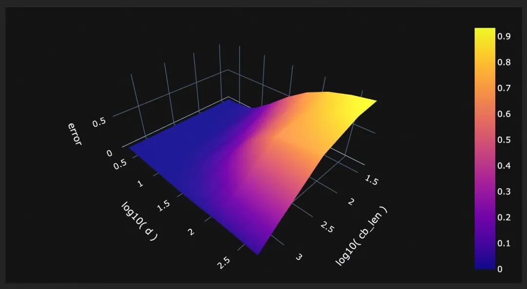
图 18. (交互式)具有不同数据维度和码本长度的4 个码本的重建误差表面图。
因此,正如我们所料,更长的码本会有所帮助,而在更高的维度上,误差往往会更大。
以下是同样的事情,但误差采用对数轴表示:
camera=dict( up=dict(x=0, y=0, z=1), center=dict(x=-0.15, y=0, z=-0.2), eye=dict(x=1.2, y=-1.4, z=1))
fig = plot_results(results, d_choices, cb_lengths, K_choices, log_xy=True, log_z=True, camera=camera)
fig.show()
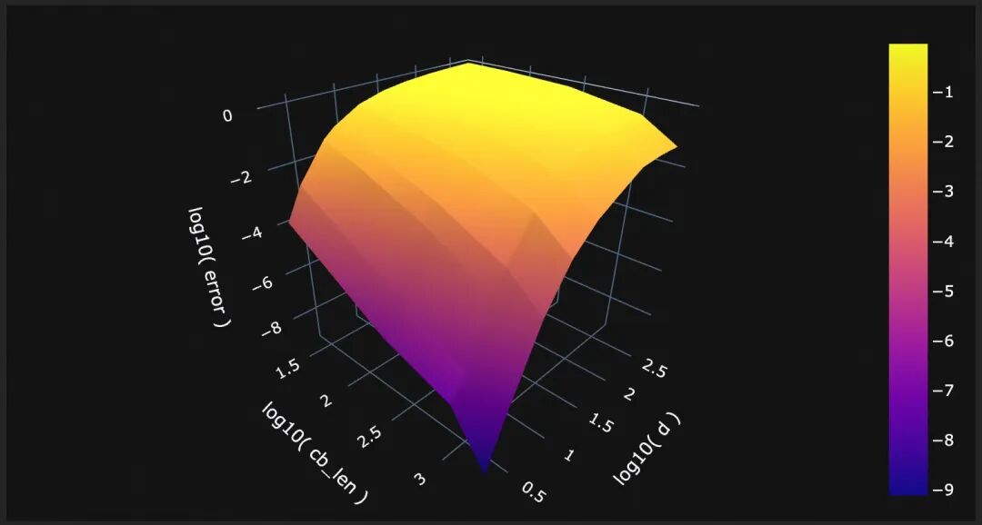
图 19. (交互式)4 个码本的重建误差表面图,每个码本包含不同的数据维度和码本长度。(z 轴为对数)
现在让我们看一下码本长度为 2048 的误差,其中我们改变了码本的数量:
camera=dict( up=dict(x=0, y=0, z=1), center=dict(x=-0.1, y=0, z=-0.22), eye=dict(x=0.3, y=-1.8, z=1))
fig = plot_results(results, d_choices, cb_lengths, K_choices, vary_K=True, log_xy=True, log_z=True, camera=camera)
fig.show()

fig, ax = plt.subplots(figsize=(6.5,4))
ourdata = results[:,-1,:] # max cb_len
for q1, d in enumerate(d_choices):
    x = np.array(K_choices)
    y = ourdata[q1]
    ax.semilogy(x,y,'o-',label=f"d = {d}")

box = ax.get_position()
ax.set_position([box.x0, box.y0, box.width * 0.8, box.height])
ax.legend(loc='center left', bbox_to_anchor=(1, 0.5))
ax.set_xlabel("K")
ax.set_ylabel("error")
plt.show()
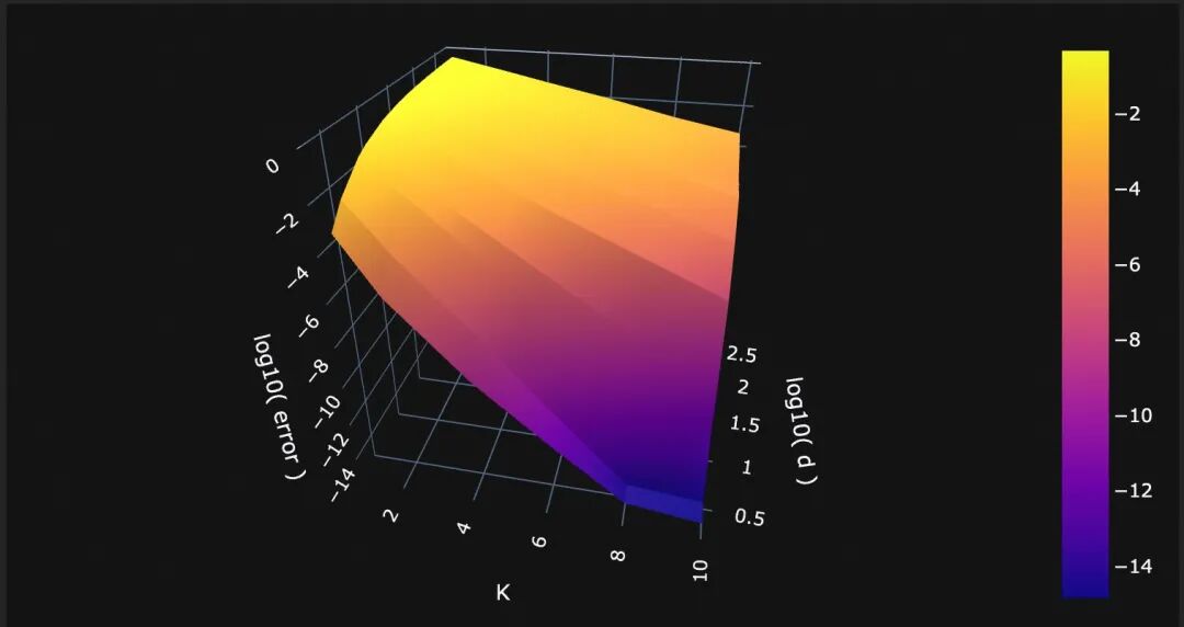
(a)(交互式)3D表面图
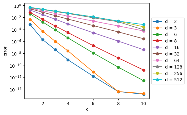
(b)线图
图 20.码本长度为 2048 时,不同数据维度和码本数量 (K) 的重构误差。(z 轴为对数)
请注意,在最后一张图中,随着 K 的变化,我们看到直线(是的,当我们达到机器精度(10^-15)时,线条就会变平, 不用担心),并且 K 轴是线性的,误差轴是对数的。这意味着——这是一个重要的结论:
大创意 当我们将码本添加到 RVQ 算法中时,错误会呈指数下降!
这是 RVQ 方法的一大“卖点”:计算成本线性增加,错误减少却获得指数级的回报。
极高维度下的难度
然而,上述结果还表明,对于非常高的维度(例如,d>=128),(R)VQ 提供的收益远不及低维度那么大 —— 添加更多更大的码本对错误没有太大影响。
因此,在他们全新的第二篇论文《使用改进的 RVQGAN 进行高保真音频压缩》中,Descript团队选择将其投影到低维空间(d=8) , 首先使用线性层,然后执行RVQ,然后使用另一组线性层投影回来。
……暂时就此打住。我们还有很多可以说的和可以做的 —— 比如,“如何使用 RVQ 进行反向传播?” —— 不过,现在看来,这个讨论应该暂时停顿一下。
致谢
感谢Harmonai的Zach Evans激励我研究这个主题,并在我写作时提供有益的讨论和纠正。
附录: AI对RVQ的解释
好的,我们来用最通俗、最生活化的方式,讲清楚“残差矢量量化”(Residual Vector Quantization, 简称 RVQ)是什么,它为什么厉害,以及它和我们日常生活的哪些东西类似。
🌟 一句话理解
残差矢量量化,就是“分步猜数字,越猜越准”的压缩技术。
它把一个复杂的数据(比如一个向量)拆成好几“步”来近似,每一步都只负责“修正上一步的误差”,最终用很少的信息,就能还原出非常接近原数据的结果。
🧩 第一步:先理解“矢量量化”(VQ)
想象你有一张非常高清的照片,像素是 1920x1080,每个像素的颜色用一个“颜色向量”表示(比如 RGB 值)。
你想把它压缩,让它变小,但又不想太模糊。
普通压缩:直接降低分辨率或扔掉一些颜色。
矢量量化(VQ):我们想个聪明办法。
我们先准备一个“颜色小字典”(叫“码本”,Codebook),里面只有 256 种颜色。比如:深红、浅蓝、墨绿……这些是“代表色”。
然后,对于照片里的每一个像素,我们不存它的精确颜色,而是存一个“编号”——这个编号指向“小字典”里的某个代表色。
例如:编号
123代表“天蓝色”。
这样,原来一个颜色要存 3 个字节(RGB),现在只存 1 个字节(编号),就实现了压缩。
但问题是:如果真实颜色是“淡天蓝”,而字典里只有“天蓝”,那就会有误差(失真)。
🔧 第二步:引入“残差”(Residual)
“残差”就是“差多少”。
比如:
- 你猜我身高是 170cm(这是你的“量化值”)。
- 但我的实际身高是 173cm。
- 那么,“残差”就是
173 - 170 = 3cm。
这个“3cm”就是你猜错的部分。
🎯 第三步:残差矢量量化(RVQ)——分步修正
RVQ 的聪明之处在于:它不指望一步到位,而是分好几步,一步步修正误差。
🧩 举个生活例子:猜价格游戏
假设你要猜一件商品的价格,比如 173.45 元。
你有一个“数字字典”,但里面只有 100 以内的整数。
❌ 普通 VQ(一步猜):
- 你只能从字典里选一个最接近的数,比如
170。 - 误差是
3.45,结果不够准。
✅ RVQ(分步猜):
- 第一轮:你从字典里选一个“大方向”的数,比如
170。- 残差 =
173.45 - 170 = 3.45
- 残差 =
- 第二轮:你再用同一个字典(或另一个小字典),去猜这个“残差”
3.45。- 你猜
3 - 新残差 =
3.45 - 3 = 0.45
- 你猜
- 第三轮:再猜
0.45,你猜0.5- 残差 =
-0.05(很小了,可以忽略)
- 残差 =
最终,你用三个“编号”(170, 3, 0.5)还原出 170 + 3 + 0.5 = 173.5,非常接近真实值 173.45。
而你只用了 3 个字典里的“代表数”相加,就实现了高精度还原。
🧠 在 AI 和数据压缩中怎么用?
在 AI 模型(比如语音、图像、向量数据库)中,数据是“高维向量”(比如一个 768 维的向量)。
直接量化会失真严重。
RVQ 的做法:
- 第一层量化:用一个码本,把 768 维向量近似成一个“粗略版本”。
- 计算残差:原向量 - 粗略版本 = 残差向量(还是 768 维,但数值小很多)。
- 第二层量化:再用一个码本,去量化这个残差向量。
- 重复:再算新残差,再量化…… 一般做 4~8 层。
最终,你只需要存储每一层“用了哪个编号”,比如 [123, 45, 67, 89]。
解码时,把每层的“代表向量”加起来,就能还原出一个非常接近原向量的结果。
✅ RVQ 的好处
优点 | 说明 |
|---|---|
压缩率高 | 只存几个编号,数据量极小 |
精度高 | 多层修正,误差越来越小 |
结构简单 | 每层都用同一个小码本,实现简单 |
适合硬件 | 适合在手机、边缘设备上运行 |
🧩 总结:用一个比喻收尾
想象你要画一幅画:
- 普通压缩:直接画个简笔画。
- 普通 VQ:用一套有限的色块拼贴,但颜色不准。
- RVQ:你先用大笔触铺底色(第一层),再用小笔触修正细节(第二层),再用更细的笔处理光影(第三层)…… 最终用很少的“笔触指令”,画出一幅非常逼真的画。
✅ 所以,残差矢量量化 就是:
“先搭架子,再修细节” 的智能压缩术,用“分步纠错”的方式,用极少的信息,还原出高质量的数据。
参考
https://drscotthawley.github.io/blog/posts/2023-06-12-RVQ.html
https://github.com/drscotthawley
本文参与 腾讯云自媒体同步曝光计划,分享自微信公众号。
原始发表:2025-09-12,如有侵权请联系 cloudcommunity@tencent.com 删除
评论
登录后参与评论
推荐阅读
目录
腾讯云开发者

Copyright © 2013 - 2026 Tencent Cloud. All Rights Reserved. 腾讯云 版权所有
深圳市腾讯计算机系统有限公司 ICP备案/许可证号:粤B2-20090059  粤公网安备44030502008569号
腾讯云计算(北京)有限责任公司 京ICP证150476号 | 京ICP备11018762号